Machine learning and the digital era from a Process Systems Engineering perspective

Texto completo

(1)Machine learning and the digital era from a Process Systems Engineering perspective* José Luis Pitarch1[ORCID](✉) and César de Prada2[ORCID] 1. Systems Engineering and Automatic Control department, EII, Universidad de Valladolid, C/Real de Burgos s/n, 47011 Valladolid, Spain [email protected] 2 Institute of Sustainable Processes (IPS), Universidad de Valladolid, C/Real de Burgos s/n, 47011 Valladolid, Spain [email protected] Abstract. Modern sensorization, communication and computational technologies provide collecting and storing huge amounts of raw data from large cyberphysical systems. These data should serve as the basis to take better decisions at all levels (from the design to operation and management). Nevertheless, raw data needs to be transformed in useful information, usually in the form of prediction models. Machine learning plays thus a key role in this task. The process industry is not alien to this digital transformation, although large processing plants present particularities that differentiate them from other systems. These differences, if neglected, can make machine learning for general purpose fail in extracting the right information from data, leading thus to unreliable process models. As such models are the basis on which the ideas towards the cognitive plant rely, this issue is of key importance for a successful full digitalization of the process industry. Here we discuss these aspects, as well as the more suitable machine-learning approaches, through our experience in an industrial case study. Keywords: machine learning, data conditioning, process modeling, data reconciliation, constrained regression, grey-box models.. 1 Introduction In the digital era, the impressing amount of data that can be stored as well as the speed at which they can be stored are expected to significantly impact the decision-making procedures at all levels of a factory: from the process design, through the operation and maintenance, to production scheduling and supply chain. Coordinating actions at all levels is the work towards reaching the full digitalized, cognitive and, ultimately, autonomous plant. However, in the process industries (those that process bulk materials or resources to transform them into products), these expected advances will not came alone by just collecting huge amounts of data and presenting them in a nice view: data treatment and analytics is necessary to ensure the data quality. Moreover models for. ∗ This research received funding from the EU Horizon 2020 research and innovation programme under. Grant No. 723575 (CoPro), and by the Spanish MICINN with FEDER funds (PGC2018-099312-B-C31)..

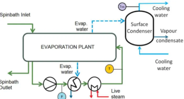
(2) 2 reliable predictions need to be build upon such data, in order to be later used in advanced control, optimization and planning routines [1]. Once data quality is ensured, models are to be build, and the current trends from the big-data revolution seem to impose the wide set of machine-learning (ML) techniques in any sector. However, as we will illustrate, the direct application of an ML approach to a modelling problem in the process industry needs to be evaluated carefully. In this particular sector, production takes place in a set of complex (and expensive) process units, linking flows of materials and energy at a large scale. Nonetheless, the process industry is not characterized by a scarce knowledge on the involved processes: researchers on Process Systems Engineering (PSE) [2] have been developing physical models (e.g., distillation columns) for design, simulation and decision-support solutions for years. Although these models have limitations for its use in real-time applications (computational complexity and/or fitness to actual plants), it is not sensible to throw out all this deep knowledge and replace it by deep-learning machines [3]. Hence, one of the key challenges of ML to successfully penetrate in the process industry is developing methods and tools that are able to naturally embed the existent physical knowledge on the underlying processes. Researchers in PSE have already taken some steps forward in this path: a) developing grey-box models (combination of first-principles laws and regression equations) which get a high matching level with the actual plant [4]; b) proposing methodologies for robust data analysis/reconciliation [5]; and c) presenting approaches/tools for datadriven modeling that are tailored to the features of the process industry [6], [7]. In the following sections, we discuss the above-mentioned issues with ML through an industrial case study that consists of building a prediction model for the fouling accumulation in the heat exchangers of a multiple-effect evaporation plant. We also test the recently proposed methodologies and software on this case, trying to give the reader a clearer vision on the potential advantages as well as the existing limitations.. 2 Description of the case study and motivation The case study is an evaporation plant in a cellulose fiber production factory, whose objective is to continuously remove certain amount of water from an acid liquid inlet (spinbath hereinafter) that comes from spinning machines, the place where cellulose pulp is recovered into fibers of desired properties. The plant layout, simplified in Fig. 1, makes use of several heat exchangers in serial connection to heat the spinbath up to a temperature suitable to start the evaporation by pressure drop. This pressure drop is first created in the evaporation chambers by induced vacuum, and later by further condensation in an attached surface condenser, creating thus a multiple-effect evaporation. The efficiency of these type of plants (livesteam consumption per amount of evaporated water) is determined by: 1) the performance of the cooling system and 2) the fouling state in the heat exchangers (due to deposition of organic residues present in the spinbath) [8]. Therefore, representative, but of limited complexity, models of these systems are needed to predict online the impact that the operation will have on the plant performance over time..

(3) 3. Fig. 1. Schema of the evaporation plant with attached surface condenser as cooling system.. For such a task, a set of experiments were performed running the plant and the cooling system in different operating conditions (setting different values for the main control variables: spinbath flow, temperature set point, cooling water flow). Moreover, in order to get information on the fouling degradation in the exchangers over time, an extensive dataset corresponding to several months of operation (including stops for cleaning) has been also recovered from the collected plant historian. In this way, the modeler may be tempted to directly try to find regression models which relate the live-steam consumption with the input variables through raw measurements. This involves some risks and limitations, as we will see later on.. 3 Data conditioning and variable estimation Everybody in the machine learning and data-analytics research community claims that ensuring the quality of data is essential to extract sensible information: process measurements need to be coherent and reliable. In industrial practice, however, it is not common to go beyond the standard filters to exclude faulty instrumentation (out of range sensors, communication loss, etc.) and to average data with the aim of mitigating the effect of noise to account for steady state in large-scale systems. A systematic method to detect and assign the quality of process data can be proposed from the Spanish AENOR-UNE norm 500540 [9], used to analyze data in meteorological stations. This method is based on several progressive levels of tests where each datum is associated to the highest quality level being passed, see Fig. 2. Note that the more restrictive tests (thus, the ones ensuring higher confidence data) are model based.. Fig. 2. Data quality validation levels..

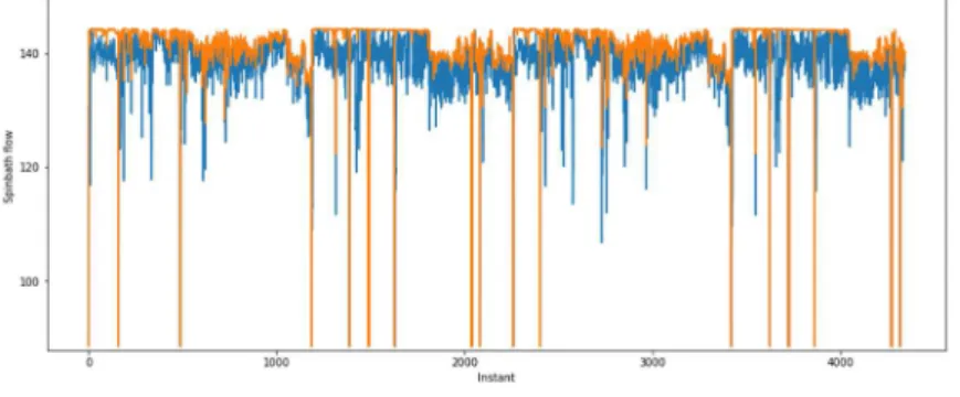
(4) 4 Each level depicted in Fig. 2 corresponds to the following quality tests: • Level 0: Communications. Check whether the data is recorded or not at an expected sampling time (problems in the sensor or in the communication system). • Level 1: Limits. Check that the datum is within instrument span and/or physical range. E.g., the maximum values expected of the flowmeters will be determined by a simple analysis of the flow capacity limit of the pipes. • Level 2: Trends. Take into account the time changes of the data in consecutive sampling times. E.g., the level in a big tank cannot change faster than several centimeters by minute. • Level 3: Data reconciliation. With a basic first-principle model of the plant, apply methods of (dynamic) data reconciliation (DR) and gross-error detection [5]. This provides a reliable set of measurements as well as estimations of unmeasured variables and parameters that are coherent with the process physics. E.g., mass balances need to be fulfilled in each time instant. • Level 4: Time series & correlations. Take into account the time series of the collected values for each variable [10]. E.g., a time-series model can be derived by analyzing the historical data of the flows in a pipe, relating them with valves, and the model output is later used to compare and to validate the newly recorded data. Fuzzy logic and set theory can be used to develop filters for the three first levels, based on comparison rules which are able to remove inconsistent data [11]. Different strategies and rules can be used, such as range and speed of change of the measurements, etc. Nevertheless, what really makes the difference in the authors’ opinion are the modelbased levels, because they include process knowledge in the data processing. Of course, these involve higher engineering effort for implementation, as relatively complex models of the plant/process (either first principles or time series) need to be previously build. After these quality tests, resource and key efficiency indicators can be defined upon reliable sets of measurements to monitor the plant efficiency in real time [12]. Instrumentation issues and DR in the evaporation plant. When retrieving sensor data from the historian, we already had to face the first issues: many of the collected flow measurements were either “upper bounded” by the instrument range (span-related issue) or they were showing higher values than the actual flow, see Fig. 3. In particular, this last problem was not caused by a biased instrument, but because of the improper location of the instrument itself: there was a bypass valve in the pipe after the flowmeter, so a (non-constant) undetermined part of the spinbath was sent to another equipment. Hence, the actual flow was usually lower. Realizing of such wrong values and the explanation took us a significant amount of time and several failed modeling attempts. However, most of these data passed the tests of range-based filters. Here we highlight the importance of the model-based tests, as suitable DR of these wrong measurements with mass-balance equations plus the rest of plant measurements provided the corrected values depicted in blue in Fig. 3. Moreover, back to the end goal of predicting the fouling in the evaporation plant, we already encounter an additional issue: the long-term loss of efficiency observed only in one output (increase of live-steam consumption) is masked with the cooling system.

(5) 5 performance and the plant operation conditions (spinbath flow). Hence, the fouling effect is hardly identifiable by a direct ML approach with the available measurements.. a) Wrong measurement due to wrong sensor placement.. b) Actual values exceeding the instrument range. Fig. 3. Flow-measurement issues. Orange line: sensor values. Blue line: actual values.. To overcome this issue, we also recalled dynamic DR [5], including the energy balances in the plant model, to estimate the lumped heat-transfer coefficient 𝑈𝐴(𝑡) in the exchangers over the time [7]. Machine-learning techniques can be now applied to “discover” models upon these coherent estimations, also called virtual measurements in the soft-sensors related literature. Details provided below.. 4 Prediction models and constrained regression Once reliable values for all process variables (states 𝑥, outputs 𝑦 and inputs 𝑢) are available, including coherent estimates of time-varying parameters and/or process unknown inputs 𝑧, any ML approach (e.g., artificial neural networks [4], canonical partial least squares [13], support vector machines [14], etc.) can be, in principle, good candidate to build plant surrogate models in the form 𝑦 = 𝑓(𝛼; 𝑥, 𝑢, 𝑧), 𝛼 ∈ ℝ regression parameters,. (1) ∗. or submodels (equations being part of a larger model) relating some variables 𝑧 ∈ 𝑧.

(6) 6 𝑧 ∗ = 𝑔(𝛽; 𝑥, 𝑢, 𝑧), 𝛽 ∈ ℝ regression parameters.. (2). At this point, there is a fundamental question to discuss: Even having reliable datasets for regression, are “standard” ML approaches enough to guarantee black-box models whose response is coherent with the process physics? Thinking on it, the answer to that question is in general NO, and the reason is given next. If you outlook the training methods by the usual ML tools, you will find that most of them rely exclusively on data, and that the performance of the black-box model to train is basically defined by the fitness to such data (plus suitable regularization to avoid overfitting, of course). In this way, although the data is coherent with the process physics (passing the tests in Section 3) and the model achieves a perfect fit to such data, there is no guarantee that its response (even with regularized smooth models) takes values that violate basic physical principles at input values not contained in the training dataset. Indeed, a model can show good statistics (R2, RMSE, etc.) in validation datasets, but it may still “predict” negative flows out of the training region (extrapolation issues) or a non-monotonic response between consecutive inputs (interpolation issues). As the end purpose of surrogate or grey-box models is to be used for decision support in (economic) control and optimization routines (hence, mainly for interpolation and extrapolation), the data-driven parts must be in coherence with the process physics [6], [15]. Therefore, some properties on the model response, such as bounds on the outputs and/or in their derivatives (monotony, curvature, convexity, etc.) would like to be ensured, not only in the regression data but in the entire expected region of operation. Thus, ML in the PSE framework needs to be extended to include additional constraints on the model, constraints which ideally need to be enforced on infinitely many points belonging to the (usually local) plant operating region. Here is where the concept of constrained regression plays a key role. 4.1 Constrained regression. Assume that a dataset of 𝑁 samples over time for some outputs 𝑦 (or, equivalently, estimations of those 𝑧 ∗ in (2)) and some inputs (𝑥, 𝑢, 𝑧) is available. Then, a candidate model for regression 𝑓(⋅) is sought such that a 𝑝-measure of the error (e.g., 𝐿 -regularized or least squares) w.r.t. the data is minimized over a set of constraints 𝑐(⋅): min ∑. 𝑦[ ] − 𝑓 𝛼; 𝑥[ ] , 𝑢[ ] , 𝑧[. ]. s. t. : 𝑐(𝛼; 𝑥, 𝑢, 𝑧) ≤ 0 ∀ 𝑥 ∈ 𝒳, 𝑢 ∈ 𝒰, 𝑧 ∈ 𝒵 𝛼∈𝒜. (3). Note that the additional constraints 𝑐(⋅) specifying some desired features on the model response is locally enforced in a compact region Ω ≔ 𝒳 ∪ 𝒰 ∪ 𝒵 of the input-space variables. These constraints may range from the more simple bounds on 𝑦 ensuring, for instance, non-negativity, to the more complex bounds on the model n-degree derivatives (slope, curvature, convexity, etc.). Defined this way, (3) is a semi-infinite constrained nonlinear optimization problem, but it can be computationally tractable under some assumptions [16]. Next, we briefly present two approaches and software available to handle (3), jointly with a discussion on their advantages and limitations..

(7) 7 Global mixed-integer approach to symbolic regression. In this approach, the functional form of the candidate regression model is assumed to be unknown a priori. Instead, the algorithm seeks to construct it from a set of predefined basis functions ℬ, e.g., ℬ ≔ {1, 𝑥, 𝑥 , 1/𝑥, log(𝑥) , 𝑒 }. Once this set is specified, the lowest complexity function 𝑓(⋅) that accurately fits the data is found from the selection of the more suitable basis in ℬ via mixed-integer programming (MIP). The idea is to split the resolution of (3) in two stages: first, solving a data-driven constrained regression (i.e., 𝑐(⋅) is only checked on the points in the dataset) and, subsequently, testing the fulfillment of constraints 𝑐(⋅) by solving a maximum-violation problem with the model already fixed from stage 1. Hence, if a point on the input space is found to violate 𝑐(⋅) with the initially proposed model, such point is virtually added to the inputs dataset and the procedure repeats until no violation of the constraints is found in stage 2 [6]. If the basis functions are chosen such that they are affine in decision variables1, typically the coefficients of a linear combination on them, then the problem to solve in stage 1 is computationally tractable (MIQP or MILP depending on the chosen norm for the regression error, i.e., 𝑝 = 1 or 𝑝 = 2). For example, for input variables 𝑥, (3) becomes: min ∑ ,. 𝑦[ ] − 𝛼 + 𝛼 𝑥[ ] + 𝛼 𝑥[ ] +. s. t. : −𝛼 − 𝛼 𝑥[ ] − 𝛼 𝑥[ ] −. [ ]. [ ]. − 𝛼 log 𝑥[. + 𝛼 log 𝑥[ ]. −𝛼 𝑒. [ ]. ]. +𝛼 𝑒. [ ]. ≤ 0 𝑡 = 1, … , 𝑁. (4). 𝐚𝐢 𝜂 ≤ 𝛼 ≤ 𝐚𝐢 𝜂 𝑖 = 0, … ,5; 𝛼 ∈ ℝ 𝜂 + 𝜂 + 𝜂 + 𝜂 + 𝜂 + 𝜂 = 𝑇; 𝜂 ∈ {0,1} In this way, the basis functions are active when the corresponding binary variable 𝜂 = 1 and inactive otherwise. Model complexity is specified by a parameter 𝑇 that is increased until a goodness-of-fit measure worsens, such as the corrected Akaike Information Criterion [17]. Afterwards, in step 2 an adaptive sampling methodology based on derivative-free global optimization techniques is used to identify points where the model is inaccurate and/or does not fulfill constraints. For the above example: max 𝛼 + 𝛼 𝑥 + 𝛼 𝑥 +. + 𝛼 log(𝑥) + 𝛼 𝑒. s. t. : 𝑥 ∈ 𝒳. (5). Note importantly that this problem is in general nonlinear and nonconvex. This procedure is what the software ALAMO implements [18]. Although this approach involves iterations between MIP and NLP problems to global optimality (time consuming), the software BARON [19] reaches acceptable computing times in many situations. Sum-Of-Squares (SOS) constrained regression. An alternative approach is casting problem (3) as a polynomial SOS optimization one [20] under mild assumptions. Of course, the main limitation of this approach is that the 1. Note that this is a strong limitation for the selection of some nonlinear basis functions in practice, like 𝑒 where its time constant 𝜏 needs to be fixed a priori, i.e., cannot be identified by the fitting algorithm..

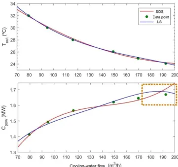
(8) 8 candidate models 𝑓(⋅) need to be polynomial in their arguments, i.e., the “potential set of basis functions” would be formed only by monomials in the input variables up to a predefined degree 𝑑. Nonetheless, paying this price worth it, because the resulting (single) optimization problem is convex, and the extra constraints on the model response and/or in its derivatives are naturally enforced (either globally, or locally in a region Ω defined by polynomial boundaries) with full guarantee of satisfaction, no matter how many samples are to be fitted or which region was covered by the experiments. In this way, high-order polynomial regressors can be used with guarantees of well-behaved resulting function approximators, compared to most options in prior literature. For instance, a SOS version of the above (4)-(5) could be: min ∑ , ,. s. t. :. 𝜙. 𝜙 𝛼 + 𝛼 𝑥[ ] + 𝛼 𝑥[ ] + 𝛼 𝑥[ ] + 𝛼 𝑥[ ] ≽ 0 𝑡 = 1, … , 𝑁; 𝜙 ∈ ℝ (∗) 1 𝛼 + 𝛼 𝑥 + 𝛼 𝑥 + 𝛼 𝑥 + 𝛼 𝑥 − 𝑠(𝛽; 𝑥) ⋅ (5 − 𝑥 ) is SOS ∀ 𝑥 ∈ ℝ 𝐚𝐢 ≤ 𝛼 ≤ 𝐚𝐢 𝑖 = 0, … ,5; 𝛼 ∈ ℝ. (6). 𝑠(𝛽; 𝑥) ≔ 𝛽 + 𝛽 𝑥 + 𝛽 𝑥 , 𝛽 ∈ ℝ, is SOS ∀ 𝑥 ∈ ℝ Here, well-known Schur complement and Positivstellensatz (see [7] for details) have been used to cast the quadratic objective function (with extra decision variables 𝜙) and the local enforcement of the constraint in a region Ω ≔ {𝑥: |𝑥| ≤ 5} (with extra decision variables 𝛽), respectively. Note that the highest degree of the polynomial SOS multipliers 𝑠(⋅) is chosen such that deg 𝑠(𝛽; 𝑥) ⋅ (5 − 𝑥 ) ≥ 𝑑. In this case, although no automatic selection of the suitable monomials among a potential set is done via MIP, note that standard regularization on the model coefficients 𝛼 can be trivially included in the objective function, for instance with a metaparameter Γ that progressively weights the coefficients corresponding to high-degree monomials. 4.2 Application to the case study. Recall from Section 2 that the aim is to get data-driven prediction models of limited complexity for the cooling system performance and the fouling in the exchangers. Modeling the cooling power provided by the surface condenser. The actual cooling power can be computed from the data collected by the temperature sensors at the water inlet (𝑇 ) and outlet (𝑇 ) of the SC, and by the flowmeter measuring the volumetric water flow (𝐹 ) send through the SC, as follows: 𝐶. =. .. 𝐹 ⋅ (𝑇. −𝑇 ). (7). Thus, what is missing to fully predict the cooling power is a model that relates the outlet temperature 𝑇 with the water flow 𝐹 and the inlet temperature 𝑇 . To model that, a polynomial candidate function up to degree 3 in 𝐹 was proposed to experimentally fit the recorded temperature difference Δ𝑇 ≔ 𝑇 − 𝑇 [21]:.

(9) 9 Δ𝑇 = 𝛼 + 𝛼 𝐹 + 𝛼 𝐹 + 𝛼 𝐹. (8). The fitting of (8) to the experimental data was done first by standard LS unconstrained regression, obtaining the resulting blue curves depicted in Fig. 4. As it can be seen, when computing the cooling power with the obtained model, it shows a behavior incoherent with the physics at high flows (remarked region in the dashed box), i.e. the cooling power cannot decrease with higher flows. However, the model fitted the measured outlet temperature (𝑇 was nearly constant during the experiments) quite well, with a monotonic response in fact, but this didn’t avoid the wrong response in 𝐶 .. Fig. 4. Fitting of the cooling power developed by the SC with different water flows.. Then, SOS constrained regression was recalled in a second attempt, adding the constraint2 d𝐶 ⁄d𝐹 > 0 to enforce the known physical knowledge on the response. Now, the obtained model (red curves in Fig. 4) behaves as expected, without showing any significant fitting degradation w.r.t the obtained by standard LS. Modeling the heat transmission in the exchangers. The goal here is to build up a model to predict both the influence of the spinbath flow 𝐹 and the operation time since last cleaning task 𝑡 (fouling effect) in the lumped heat-transfer coefficient 𝑈𝐴. Here we make use of the 𝑈𝐴 estimations provided by DR, already mentioned in Section 3 (omitted for brevity, see [7]). The first issue arose when selecting sets for training and validation: although the recorded dataset looked huge (plant historian of 7-months length at 5-min. sampling time), 2. Note that derivatives of polynomials are also polynomials that can be directly checked for SOS..

(10) 10 the plant was usually running at high flows. Therefore, a significant amount of information of the convection and fouling behaviors at medium/low flows was missing. In order to palliate this issue, few experiments were executed on purpose when possible (normally one is not allowed to “play” with an industrial plant in continuous production). Consequently, as often happens in the process industry, we ended up doing “bigdata stuff” with subsets of 22 samples for training plus 20 for validation, depicted in the figures below. This is nearly all the information available in the region of operation. With this material, if no additional information about the process physics is included in the fitting problem, standard ML techniques fail in obtaining reliable black-box models in the regions where there is a lack of data to fit. See for instance problems of overfitting with standard LS in Fig. 5a, and problems of abrupt-falling responses (even going negative) where data is missing in Fig. 5b, despite using regularization techniques.. 1000. UA(kW/K). 800. 600. 400. 200. 0 0 10. 200. 20. 180. 30. 160. 40. Time (days). 140 50. 120 60. 100. F(m3/h). a) Least Squares. b) LS with regularization. Fig. 5. Fitting of the heat-transmission coefficient by standard ML methods.. a) Model by ALAMO. b) Model by polynomial SOS. Fig. 6. Fitting of the heat-transmission coefficient by constrained regression.. On the contrary, constrained regression in Section 4.1 fixed these modeling issues. We tested the “ALAMO approach” with a large set of basis functions including monomials.

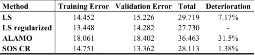
(11) 11 up to degree 4, rational powers, square roots, logarithms and exponentials. We also set up the additional constraint 𝑓 𝛼; 𝐹 , 𝑡 > 200 in the local-input region Ω. Thus, choosing the Akaike’s criterion to avoid overfitting, we got the model (Fig. 6a): 𝑈𝐴 = 2.27𝐹. − 0.9095𝑡. (9). + 84.978 log(𝐹 ) − 42.525 𝑡. Going by the way of SOS constrained regression, proposing a candidate polynomial model with highest degree 𝑑 = 4 and setting (local) bounds on its partial derivatives ;. 0<. ,. < 𝜆 , −𝜆 <. ;. ,. < 0, ∀ 𝐹 , 𝑡. ∈Ω. (10). to enforce a smooth and physically-coherent response, the model of Fig. 6b is got [7]: 𝑈𝐴 = 7.06e 𝐹 + 2.95e 𝐹 𝑡 + 1.63e 𝐹 𝑡 − 2.42e 𝐹 𝑡 + 1e 𝑡 2e 𝐹 − 1.585e 𝐹 𝑡 + 5.1e 𝐹 𝑡 − 0.0138𝑡 + 0.089𝐹 + 0.232𝐹 𝑡 + 0.627𝑡 − 10.87𝐹 − 22.78𝑡 + 1000. −. (11). Note that the model (11) got by SOS constrained regression keeps the desired physical features without incurring in significant fitness deterioration w.r.t. “the best” obtained by unconstrained LS regression with regularization, see the table below. Table 1. Absolute LS error accumulated by the presented models. Method Training Error Validation Error LS 14.452 15.226 LS regularized 13.448 14.282 ALAMO 18.061 18.402 SOS CR 14.751 13.362. Total Deterioration 29.719 7.17% 27.730 36.463 31.5% 28.113 1.38%. 5 Final remarks In this paper, we have discussed how essential is incorporating process knowledge beyond sampled data in order to really extract sensible information, which can be later use for decision support. For this task, model-based tests to detect (and improve) the data quality (robust DR methods in particular) as well as constrained-regression approaches proven to be quite effective in our case study. Constrained regression is especially relevant/useful when few samples are available, or when there are lots of samples but containing nearly the same information about the process. It is also worth to remark that incoherent model responses could be detected (and corrected ad-hoc perhaps) in two or three-dimensional models, but this would be impossible in larger multidimensional systems.. References [1]. S. Krämer and S. Engell, Eds., Resource efficiency of processing plants: monitoring and improvement. Weinheim: Wiley-VCH, 2018..

(12) 12 [2] [3] [4] [5] [6] [7] [8]. [9] [10] [11] [12] [13] [14] [15] [16] [17] [18] [19] [20] [21]. I. E. Grossmann and I. Harjunkoski, “Process systems Engineering: Academic and industrial perspectives,” Comput. Chem. Eng., vol. 126, pp. 474–484, Jul. 2019. I. H. Witten, E. Frank, and M. A. Hall, Data mining: practical machine learning tools and techniques, 3rd ed. Burlington, MA: Morgan Kaufmann, 2011. L. F. M. Zorzetto, R. M. Filho, and M. R. Wolf-Maciel, “Processing modelling development through artificial neural networks and hybrid models,” Comput. Chem. Eng., vol. 24, no. 2–7, pp. 1355–1360, Jul. 2000. C. de Prada and D. Sarabia, “Data Pre-treatment,” in Resource Efficiency of Processing Plants, S. K. Krämer and S. E. Engell, Eds. Weinheim, Germany: Wiley-VCH Verlag GmbH & Co. KGaA, 2018, pp. 181–210. A. Cozad, N. V. Sahinidis, and D. C. Miller, “A combined first-principles and data-driven approach to model building,” Comput. Chem. Eng., vol. 73, pp. 116–127, Feb. 2015. J. Pitarch, A. Sala, and C. de Prada, “A Systematic Grey-Box Modeling Methodology via Data Reconciliation and SOS Constrained Regression,” Processes, vol. 7, no. 3, p. 170, Mar. 2019. J. L. Pitarch, C. G. Palacín, A. Merino, and C. de Prada, “Optimal Operation of an Evaporation Process,” in Modeling, Simulation and Optimization of Complex Processes HPSC 2015, H. G. Bock, H. X. Phu, R. Rannacher, and J. P. Schlöder, Eds. Cham: Springer International Publishing, 2017, pp. 189–203. AENOR, Automatic weather stations networks: Guidance for the validation of the weather data from the station networks. Real time validation. 2004. J. Blanch, V. Puig, J. Saludes, and J. Quevedo, “ARIMA Models for Data Consistency of Flowmeters in Water Distribution Networks,” IFAC Proc. Vol., vol. 42, no. 8, pp. 480– 485, 2009. M. Last and A. Kandel, “Automated Detection of Outliers in Real-World Data,” in Proc. of the Second International Conference on Intelligent Technologies, 2001, pp. 292–301. M. Kujanpää et al., Successful Resource Efficiency Indicators for process industries: Stepby-step guidebook. Espoo: VTT Technical Research Centre of Finland, 2017. U. G. Indahl, K. H. Liland, and T. Naes, “Canonical partial least squares-a unified PLS approach to classification and regression problems,” J. Chemom., vol. 23, no. 9, pp. 495– 504, Sep. 2009. W. Yan, H. Shao, and X. Wang, “Soft sensing modeling based on support vector machine and Bayesian model selection,” Comput. Chem. Eng., vol. 28, no. 8, pp. 1489–1498, Jul. 2004. H. J. A. F. Tulleken, “Grey-box modelling and identification using physical knowledge and bayesian techniques,” Automatica, vol. 29, no. 2, pp. 285–308, Mar. 1993. O. Stein, Bi-Level Strategies in Semi-Infinite Programming, vol. 71. Boston, MA: Springer US, 2003. C. M. Hurvich and C.-L. Tsai, “A corrected Akaike information criterion for vector autoregressive model selection,” J. Time Ser. Anal., vol. 14, no. 3, pp. 271–279, May 1993. Z. T. Wilson and N. V. Sahinidis, “The ALAMO approach to machine learning,” Comput. Chem. Eng., vol. 106, pp. 785–795, Nov. 2017. N. V. Sahinidis, “BARON: A general purpose global optimization software package,” J. Glob. Optim., vol. 8, no. 2, pp. 201–205, Mar. 1996. A. Papachristodoulou, J. Anderson, G. Valmorbida, S. Prajna, P. Seiler, and P. Parrilo, “SOSTOOLS: Sum of squares optimization toolbox for MATLAB.” 2013. M. P. Marcos, J. L. Pitarch, C. de Prada, and C. Jasch, “Modelling and real-time optimisation of an industrial cooling-water network,” in 22nd Inter. Conf. on System Theory, Control and Computing (ICSTCC), Sinaia, 2018, pp. 591–596..

(13)