Chemical Abundances of Main sequence, Turnoff, Subgiant, and Red Giant Stars from APOGEE Spectra I Signatures of Diffusion in the Open Cluster M67
19
0
0
Texto completo
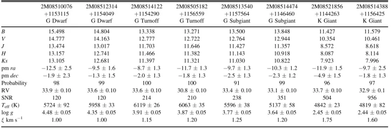
(2) The Astrophysical Journal, 857:14 (19pp), 2018 April 10. Souto et al. Table 1 Atmospheric Parameters. B V J H Ks pm ra pm dec Probability RV SNR Teff (K) log g ξ km s−1. 2M08510076 +1153115 G Dwarf. 2M08512314 +1154049 G Dwarf. 2M08514122 +1154290 G Turnoff. 2M08505182 +1156559 G Turnoff. 2M08513540 +1157564 G Subgiant. 2M08514474 +1146460 G Subgiant. 2M08521856 +1144263 K Giant. 2M08514388 +1156425 K Giant. 15.498 14.777 13.474 13.157 13.105 −12.5±2.5 −1.9±2.3 98 33.9±0.10 120 5724±92 4.48±0.05 1.00. 14.804 14.163 13.017 12.741 12.681 −9.5±1.6 −1.3±1.5 99 33.6±0.10 120 5958±33 4.35±0.05 1.00. 13.338 12.777 11.703 11.466 11.397 −8.7±1.3 −2.0±1.3 100 33.6±0.10 214 6119±26 3.91±0.05 1.15. 13.271 12.722 11.646 11.382 11.321 −11.7±1.3 −1.8±1.3 100 30.8±0.10 210 6063±35 3.87±0.05 1.20. 13.500 12.764 11.427 11.143 11.030 −9.7±1.3 −2.5±1.3 91 33.4±0.10 238 5596±38 3.77±0.05 1.25. 13.848 12.944 11.357 10.918 10.822 −10.3±1.2 −2.3±1.2 99 33.1±0.10 351 5137±58 3.64±0.05 1.20. 11.427 10.354 8.572 8.087 7.923 −11.9±1.5 −4.9±1.5 96 33.7±0.10 504 4842±23 2.45±0.05 1.75. 11.579 10.461 8.618 8.114 7.996 −9.7±2.5 −1.8±1.3 97 32.9±0.1 956 4819±82 2.44±0.05 1.60. compositions). Quantitative high-resolution spectroscopic analyses can be used to reveal if there are chemical abundance differences between the M67 members in the different evolutionary phases, as well as determining whether these differences are real or if they reveal systematic differences induced by the analysis techniques themselves. Accurate chemical abundances of a large number of elements can be used to test models of chemical diffusion in stars (e.g., Michaud et al. 2015). The recent studies by Önehag et al. (2014), Blanco-Cuaresma et al. (2015), and Bertelli Motta et al. (2017) find chemical inhomogeneities for some elements that could be an indication that diffusion mechanisms may be at work and detectable in M67 stars. Chemical abundance variations that result from diffusion have been probed in the metal-poor globular cluster NGC 6397 ([Fe/H]=−2.1) in a series of papers by Korn et al. (2007), Lind et al. (2008), and Nordlander et al. (2012). These papers studied cluster stars at the turnoff point (TOP), on the SGB, at the base of the red giant branch (bRGB), and on the RGB using chemical abundances of Li, Mg, Ca, Ti, Cr, and Fe. Chemical abundances were found to be dependent on evolutionary stage, and these were compared to diffusion models, with overall approximate agreement between observed and model abundances, particularly for Mg and Fe. Diffusion model predictions specific to the solar metallicity and age regime of M67 have been presented by Michaud et al. (2004) and most recently by Dotter et al. (2017). In both studies, diffusion effects near the turnoff in M67 have been found to be as large as ∼0.1 dex when compared to cooler main-sequence stars or stars on the RGB (where convection erases the abundance patterns created by diffusion), especially for certain elements such as Fe or Mg. Specific patterns in the abundance distributions of certain elements, such as Ca and Fe, are also predicted to exhibit detectable variations, suggesting that M67 is a key open cluster in which to probe and test models of diffusion processes. In this study, a small sample of M67 members that were observed as part of the Apache Point Observatory Galactic Evolution Experiment (APOGEE; Majewski et al. 2017) survey are analyzed using its high-resolution, near-infrared (NIR) spectra to derive accurate chemical abundances for a large number of elements. The studied sample spans a range of evolutionary phases consisting of G dwarfs, G turnoff stars,. G subgiants, and K giants. The detailed chemical abundances derived for these stars are used to investigate possible abundance inhomogeneities in M67 as a function of stellar class and determine whether such abundance variations can be explained by a physical process, such as diffusion in the stellar envelope, or reflect systematic effects associated with the analysis techniques. The recent studies of Bovy (2016) and Price-Jones & Bovy (2018) using APOGEE spectra found the tightest constraints on the chemical homogeneity of M67 red giants. This evidence of chemical homogeneity in red giants is an important starting point to investigate possible diffusion effects and assign observed abundance differences to the effects of stellar evolution. Section 2 discusses the details of the APOGEE survey and spectra, while Section 3 presents the determination of stellar parameters (effective temperature, Teff, and surface gravity, log g), along with the chemical abundances. The chemical abundance distributions and possible variations are discussed in Sections 4 and 5, with the summary of results in Section 6. 2. The APOGEE Spectra and the Sample The spectra analyzed in this work are from the SDSS-IV/ APOGEE2 survey (Blanton et al. 2017, Majewski et al. 2017). The APOGEE instrument is a cryogenic multifiber spectrograph (300 fibers; Wilson et al. 2010) on the SDSS 2.5 m telescope at the Apache Point Observatory (Gunn et al. 2006). The survey observations consist of high-resolution (R= λ/Δλ ∼ 22,500) spectra of stars, primarily red giants but also stars in other evolutionary stages (see Zasowski et al. 2013), in the NIR (∼λ1.50–λ1.70 μm) with the ultimate goal of exploring the chemical evolution of the stellar populations in the Milky Way. Our sample contains eight stars that are deemed to be members of the M67 open cluster. The APOGEE spectra of the sample stars were reduced automatically by the APOGEE pipeline (Holtzman et al. 2015; Nidever et al. 2015) and then analyzed manually to extract detailed chemical abundances. We selected targets strategically to sample a range in effective temperatures and surface gravities that are representative of stars on the main sequence and in more advanced phases of evolution: two G dwarfs, two G-type turnoff stars, two G-type subgiants, and two K-type red giants. All targets are in the 2.
(3) The Astrophysical Journal, 857:14 (19pp), 2018 April 10. Souto et al.. Figure 1. 2MASS color–magnitude diagram of the APOGEE targets in the M67 field (shown as gray dots). The red symbols correspond to the studied stars: solar-like stars (red diamonds), turnoff stars (red squares), subgiant stars (red triangles), and red clump stars (red circles). Two isochrones for an age of 4 Gyr, (m–M)0=9.60, and [Fe/H]=0.00 from PARSEC (black line) and MIST (blue line) are also shown.. proper-motion study of Yadav et al. (2008) and have probabilities of membership higher than 91% (Table 1). Their measured radial velocities from the APOGEE spectra are also presented in Table 1, and these are consistent with probable cluster membership (Geller et al. 2015). Figure 1 shows the color–magnitude diagram for the NIR 2MASS data (Skrutskie et al. 2006), with H0 plotted versus (J–Ks)0. The eight target stars are shown as filled red symbols. We also show, as gray dots, the 536 stars from the M67 field observed by APOGEE (which include additional M67 members) and two isochrones for an age of 4 Gyr, (m–M)0=9.60, and [Fe/H]=0.00 from PARSEC (Bressan et al. 2012) and MIST (Choi et al. 2016; Dotter 2016).. abundance analysis described in this section provides independent results for a small sample that can be compared to the automated ASPCAP results for a larger sample of M67 members. 3.1. Effective Temperatures The effective temperatures for the stars in the studied sample were derived using the photometric calibrations of González-Hernández & Bonifacio (2009) and five different colors (B – V, V – J, V – H, V – Ks, and J – Ks) while adopting a solar metallicity. The individual magnitudes B and V were taken from Yadav et al. (2008), and the infrared colors are from the 2MASS catalog (Skrutskie et al. 2006). A reddening E(B – V )=0.041 (Taylor 2007; Sarajedini et al. 2009) was adopted with individual dereddened colors obtained using the relations from Schlegel et al. (1998) and Carpenter (2001). The adopted colors and derived effective temperatures, plus the standard deviations of the mean (typically below ∼50 K), are presented in Table 1. When the internal uncertainties in the González-Hernández & Bonifacio (2009) calibration are included, along with the errors in the photometric colors, the total estimated uncertainty expected in Teff is ∼100 K, adding all of the errors in quadrature.. 3. Chemical Abundance Analysis The sample studied here contains a mixture of stellar types. Both of the K giants in the sample were found to be red clump (RC) giants by Stello et al. (2016) based on K2 asteroseismology. In addition, Stello et al. (2016) analyzed the K2 oscillations from one of the stars, 2M08511474+1146460, and confirmed it to be a subgiant star very close to the base of the RGB. The spectra of all eight stars were analyzed for chemical abundances in a homogeneous way that is independent from the methodology adopted in the derivation of stellar parameters and chemical abundances for the 14th SDSS Data Release (DR14) using the APOGEE automatic abundance pipeline ASPCAP (García Pérez et al. 2016). The “boutique” manual. 3.2. Surface Gravities Stellar surface gravities (log g) were derived from the fundamental relation with stellar mass, Teff, and absolute 3.
(4) The Astrophysical Journal, 857:14 (19pp), 2018 April 10. Souto et al.. bolometric magnitude (Equation (1) below). Stellar masses were estimated by using the absolute magnitudes for the B, V, H, J, and Ks filters, along with an adopted PARSEC isochrone for an age=4.0 Gyr, [Fe/H]=0.0, and (m–M)0=9.60, with derived masses then being ∼1.34 Me for the RC, ∼1.30 Me for the subgiants, ∼1.20 Me for the turnoff stars, and ∼1.00 Me for the solar-like stars. We note that if the isochrone from MIST (Figure 1) is adopted, the obtained stellar masses are not significantly different. The combination of effective temperature, stellar mass, and bolometric magnitudes (with bolometric corrections from Montegriffo et al. 1998) in Equation (1) provides the surface gravity values listed in Table 1. The solar values used were log ge=4.438 dex, Teff,e=5772 K, and Mbol,e=4.75, which follows the IAU prescription in Prša et al. (2016): ⎛T ⎞ ⎛M ⎞ log g = log g + log ⎜ ⎟ + 4 log ⎜ ⎟ ⎝ T ⎠ ⎝ M ⎠ + 0.4 (Mbol, - Mbol, ).. elemental abundance varied, until the differences between the observed and synthetic spectra were minimized. The instrumental resolution of the APOGEE spectrograph (R∼22,500) produces an instrumental profile with an ∼13.7 km s−1 full-width at halfmaximum (FWHM∼0.71 Å). Small variations in the broadening result in small adjustments across the spectra of about ∼±1.5 km s−1. During the line-profile fitting, searches were made for extra-broadening effects related to v sin(i) and/or macroturbulence; however, no extra line broadening was needed beyond the instrumental APOGEE profile to obtain good fits to the observed line profiles. Chemical abundances of the elements C, N, O, Na, Mg, Al, Si, K, Ca, Ti, V, Cr, Mn, and Fe were derived for the two RC giants in our sample (Table 2). The selected transitions were the same as in our previous study of red giants in the open cluster NGC 2420 using APOGEE spectra (Souto et al. 2016). Souto et al. (2016) analyzed a sample of red giants with similar values of Teff and log g (although slightly more metal-poor, with [Fe/H]=−0.20) to those of the M67 RC giants studied here. The previous work on NGC 2420 by Souto et al. (2016) did not analyze solar-like dwarfs, turnoff stars, or subgiants. In this study, we have made a careful search for usable spectral lines or features in the APOGEE spectra of dwarfs and subgiants, with the goal being to maximize the number of lines available for each chemical species. Initial identification of promising spectral lines in solar-like dwarfs was done using an APOGEE spectrum of the asteroid Vesta (as a solar proxy), which were observed using the APOGEE spectrograph fiber-linked to the APO 1 m telescope. The atomic and molecular lines used in the “boutique” abundance analysis of the stars (and their associated abundances) are listed in Table 2. A total of 135 spectral lines or features were selected as abundance indicators: 77 Fe I, 4 CO, 3 C I, 10 CN, 4 OH, 2 Na I, 6 Mg I, 3 Al I, 9 Si I, 2 K I, 4 Ca I, 6 Ti I, 1 V I, 1 Cr I, and 3 Mn I. As the studied sample covers an extended range in Teff–log g parameter space, it is not possible to measure the exact same transitions for all stars, given that the strengths of the various spectral features change as a function of Teff and log g. The APOGEE spectra of cool red giants are typically dominated by molecular features (mostly CO, CN, and OH) but also show atomic lines from many elements. For G dwarfs and subgiants with higher effective temperatures, molecular absorption becomes less important, and neutral atomic lines become dominant. In the case of G dwarfs and turnoff stars, it is not possible to derive oxygen and nitrogen abundances, as the molecular OH and CN lines become too weak. Vanadium abundances are also not measurable. Most chemical abundances from APOGEE are based on transitions of neutral atomic lines and include Fe, Na, Al, Mg, Si, K, Ca, Ti, V, Cr, and Mn. These lines can be measured, for the most part, in all four stellar classes, although for some lines, the degree of blending and/or the line strengths change significantly depending on the stellar class. Concerning iron, often taken as a metallicity indicator, a relatively small number of clean Fe I lines can be analyzed in red giants, while more than 70 Fe I lines can be used in the warmer subgiants, turnoff stars, and G dwarfs. Although the CO lines become quite weak for solartype stars, three C I lines (λ15784.7, λ16005.0, and λ16021.7) become stronger and measurable in these stars. Figure 2 illustrates the observed and best-fit synthetic spectra for one star in each class: one RC, one subgiant, one turnoff star, and one solar-like G dwarf (top to bottom). These spectra. (1 ). Estimates of the uncertainties in the surface gravities were computed from two isochrones with ages of 3.5 and 4.5 Gyr that were used to rederive the stellar masses. Included in these estimates were the effective temperature uncertainties, as well as a typical metallicity uncertainty of±0.05 dex. Errors in the photometric magnitudes are small and of the order of 0.03 mag. Combining all of these values in quadrature, an uncertainty of ∼0.07 dex is found for the derived values of log g. Our sample includes three stars with asteroseismic log g from the K2 mission reported in Stello et al. (2016). Our derived log g values agree quite well with the asteroseismic ones; δlogg (this work; Stello et al. 2016)=0.04±0.07 dex. 3.3. Chemical Abundances and Selected Lines Chemical abundances were derived from a 1D LTE analysis and spectral synthesis using the Turbospectrum code (Alvarez & Plez 1998; Plez 2012) in combination with model atmospheres interpolated from the MARCS21 grid (Gustafsson et al. 2008) for the atmospheric parameters derived in Sections 3.1 and 3.2 (Table 1). The APOGEE line list used in all computations was an updated version of the DR14 line list (line list 20170418). Shetrone et al. (2015) provided details on the construction of the APOGEE line list, and updates can be found in J. Holtzman et al. (2018, in preparation). In a 1D abundance analysis, the microturbulent velocity (ξ) is a necessary parameter to have both weak and strong lines of a given species yield the same abundance. Microturbulent velocities were determined using the same procedure as in Souto et al. (2016; or Smith et al. 2013). The determination of ξ relies on Fe I lines that span a range of line strengths (or equivalent widths), with the stronger lines displaying a much larger sensitivity of the derived abundance with the microturbulent velocity. The best value of ξ yields the closest agreement in the abundances of the strong and weak lines. In practice, adopted values of ξ were varied from 0.5 to 3.0 km s−1. The inferred values of ξ are included in Table 1. Chemical abundances of individual elements were derived using a line-by-line manual analysis and obtaining best fits of synthetic spectra to observed line profiles. Local continuum levels in the observed spectra were set manually, and the particular 21. marcs.astro.uu.se. 4.
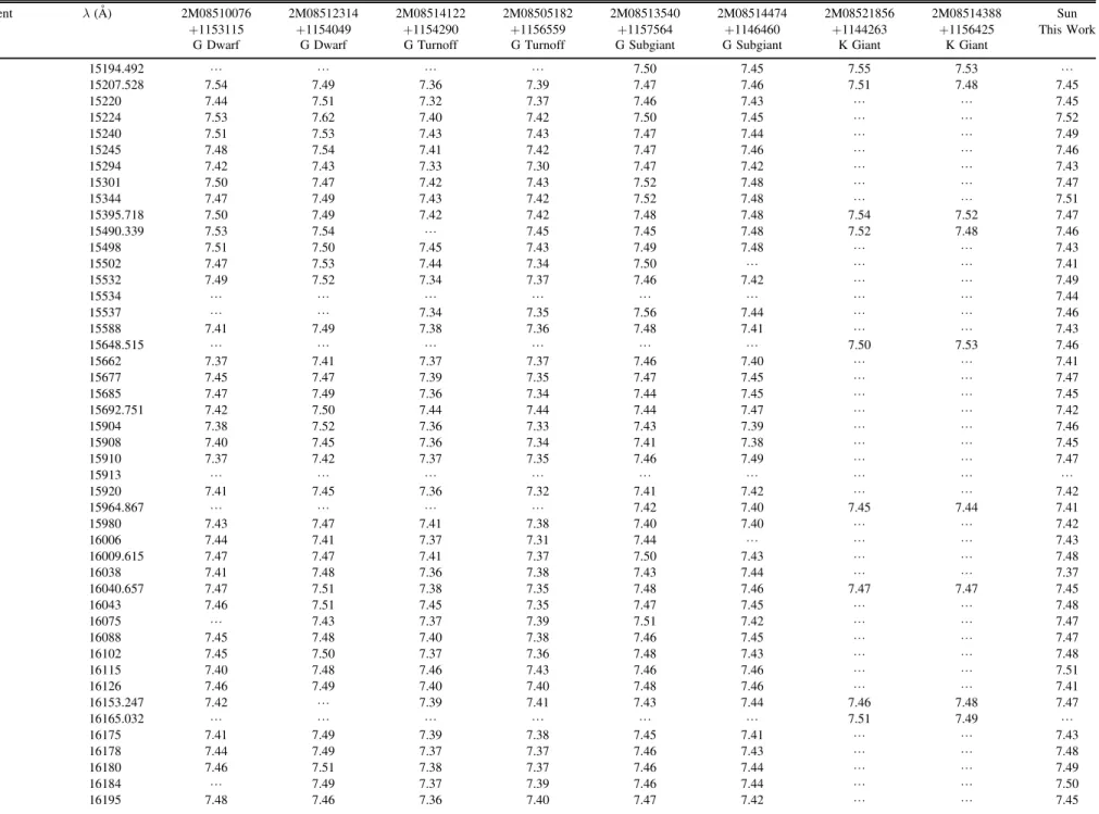
(5) Element. Fe I. λ (Å). 5. 2M08512314 +1154049 G Dwarf. 2M08514122 +1154290 G Turnoff. 2M08505182 +1156559 G Turnoff. 2M08513540 +1157564 G Subgiant. 2M08514474 +1146460 G Subgiant. 2M08521856 +1144263 K Giant. 2M08514388 +1156425 K Giant. Sun This Work. L 7.54 7.44 7.53 7.51 7.48 7.42 7.50 7.47 7.50 7.53 7.51 7.47 7.49 L L 7.41 L 7.37 7.45 7.47 7.42 7.38 7.40 7.37 L 7.41 L 7.43 7.44 7.47 7.41 7.47 7.46 L 7.45 7.45 7.40 7.46 7.42 L 7.41 7.44 7.46 L 7.48. L 7.49 7.51 7.62 7.53 7.54 7.43 7.47 7.49 7.49 7.54 7.50 7.53 7.52 L L 7.49 L 7.41 7.47 7.49 7.50 7.52 7.45 7.42 L 7.45 L 7.47 7.41 7.47 7.48 7.51 7.51 7.43 7.48 7.50 7.48 7.49 L L 7.49 7.49 7.51 7.49 7.46. L 7.36 7.32 7.40 7.43 7.41 7.33 7.42 7.43 7.42 L 7.45 7.44 7.34 L 7.34 7.38 L 7.37 7.39 7.36 7.44 7.36 7.36 7.37 L 7.36 L 7.41 7.37 7.41 7.36 7.38 7.45 7.37 7.40 7.37 7.46 7.40 7.39 L 7.39 7.37 7.38 7.37 7.36. L 7.39 7.37 7.42 7.43 7.42 7.30 7.43 7.42 7.42 7.45 7.43 7.34 7.37 L 7.35 7.36 L 7.37 7.35 7.34 7.44 7.33 7.34 7.35 L 7.32 L 7.38 7.31 7.37 7.38 7.35 7.35 7.39 7.38 7.36 7.43 7.40 7.41 L 7.38 7.37 7.37 7.39 7.40. 7.50 7.47 7.46 7.50 7.47 7.47 7.47 7.52 7.52 7.48 7.45 7.49 7.50 7.46 L 7.56 7.48 L 7.46 7.47 7.44 7.44 7.43 7.41 7.46 L 7.41 7.42 7.40 7.44 7.50 7.43 7.48 7.47 7.51 7.46 7.48 7.46 7.48 7.43 L 7.45 7.46 7.46 7.46 7.47. 7.45 7.46 7.43 7.45 7.44 7.46 7.42 7.48 7.48 7.48 7.48 7.48 L 7.42 L 7.44 7.41 L 7.40 7.45 7.45 7.47 7.39 7.38 7.49 L 7.42 7.40 7.40 L 7.43 7.44 7.46 7.45 7.42 7.45 7.43 7.46 7.46 7.44 L 7.41 7.43 7.44 7.44 7.42. 7.55 7.51 L L L L L L L 7.54 7.52 L L L L L L 7.50 L L L L L L L L L 7.45 L L L L 7.47 L L L L L L 7.46 7.51 L L L L L. 7.53 7.48 L L L L L L L 7.52 7.48 L L L L L L 7.53 L L L L L L L L L 7.44 L L L L 7.47 L L L L L L 7.48 7.49 L L L L L. L 7.45 7.45 7.52 7.49 7.46 7.43 7.47 7.51 7.47 7.46 7.43 7.41 7.49 7.44 7.46 7.43 7.46 7.41 7.47 7.45 7.42 7.46 7.45 7.47 L 7.42 7.41 7.42 7.43 7.48 7.37 7.45 7.48 7.47 7.47 7.48 7.51 7.41 7.47 L 7.43 7.48 7.49 7.50 7.45. Souto et al.. 15194.492 15207.528 15220 15224 15240 15245 15294 15301 15344 15395.718 15490.339 15498 15502 15532 15534 15537 15588 15648.515 15662 15677 15685 15692.751 15904 15908 15910 15913 15920 15964.867 15980 16006 16009.615 16038 16040.657 16043 16075 16088 16102 16115 16126 16153.247 16165.032 16175 16178 16180 16184 16195. 2M08510076 +1153115 G Dwarf. The Astrophysical Journal, 857:14 (19pp), 2018 April 10. Table 2 Individual Abundances.
(6) Element. λ (Å). 6. 16197 16199 16204 16207 16213 16232 16235 16246 16294 16315 16324 16332 16395 16398 16404 16487 16506 16516 16519 16522 16525 16531 16542 16552 16560 16612 16645 16653 16657 16661 16664 CO. 15570–15600 15970–16010 16184 16600–16650. 2M08510076 +1153115 G Dwarf. 2M08512314 +1154049 G Dwarf. 2M08514122 +1154290 G Turnoff. 2M08505182 +1156559 G Turnoff. 2M08513540 +1157564 G Subgiant. 2M08514474 +1146460 G Subgiant. 2M08521856 +1144263 K Giant. 2M08514388 +1156425 K Giant. Sun This Work. 7.53 7.49 7.40 7.53 7.46 L 7.46 7.47 7.52 L 7.43 L 7.50 7.51 7.50 7.42 7.53 7.47 7.50 7.47 7.47 7.51 7.45 7.46 7.48 7.49 7.52 7.52 7.48 7.53 7.48. 7.52 7.49 7.47 7.48 7.48 7.49 7.49 7.47 L 7.51 7.51 L 7.54 L 7.53 7.41 L 7.53 7.50 7.52 7.48 7.57 L 7.47 L 7.48 7.49 7.51 7.54 L 7.52. 7.46 7.45 L 7.40 7.45 7.40 7.38 7.40 7.37 7.41 7.33 7.43 L 7.44 7.43 7.38 7.44 7.39 7.40 7.39 7.38 7.42 7.45 7.45 7.45 7.32 7.43 7.41 7.42 7.44 7.41. 7.35 7.44 L 7.36 7.38 7.37 7.38 7.36 7.39 7.36 7.36 7.46 7.38 L 7.41 7.39 7.41 7.40 7.40 7.39 7.36 7.38 7.43 7.38 7.41 7.40 7.38 7.39 7.43 7.45 7.38. 7.44 7.44 7.42 7.44 7.48 7.39 7.47 7.45 7.44 7.42 7.48 7.48 7.48 7.49 7.49 7.43 7.52 7.45 7.49 7.51 7.50 7.49 7.48 7.49 7.49 7.48 7.49 7.46 7.50 7.54 7.49. 7.40 7.42 7.40 7.40 7.45 7.44 L 7.47 7.50 7.45 7.44 7.45 7.47 7.47 7.44 7.45 7.44 7.43 7.42 7.46 7.43 7.42 7.43 7.43 7.41 7.43 7.43 7.45 7.47 7.49 7.44. L L L L L L L L L L L L L L L L L L L L L L L L L L L L L L L. L L L L L L L L L L L L L L L L L L L L L L L L L L L L L L L. 7.52 7.48 7.43 7.41 7.45 7.42 7.42 7.46 7.47 7.45 7.43 7.52 7.48 7.46 7.49 7.37 7.47 7.44 7.45 7.46 7.44 7.48 7.45 7.41 7.40 7.45 7.47 7.44 7.47 7.43 7.49. L L L L. L L L L. L L L L. L L L L. 8.31 L L L. 8.33 L L L. 8.34 8.35 8.33 L. 8.39 8.37 8.35 L. L L L L. 15784.7 16005.0 16021.7. 8.41 8.40 8.41. 8.40 8.37 8.41. 8.26 8.28 8.31. 8.27 8.36 8.36. 8.31 8.42 8.34. 8.34 8.48 L. L L L. L L L. 8.31 8.37 8.44. CN. 15260. 15322. 15397. 15332. 15410.. L L L L L. L L L L L. L L L L L. L L L L L. 8.15 L 8.04 L L. 7.95 7.93 8.02 L 7.93. 8.03 8.16 8.17 8.10 8.15. 8.05 8.05 8.07 8.07 8.09. L L L L L. Souto et al.. CI. The Astrophysical Journal, 857:14 (19pp), 2018 April 10. Table 2 (Continued).
(7) Element. λ (Å). 2M08514122 +1154290 G Turnoff. 2M08505182 +1156559 G Turnoff. 2M08513540 +1157564 G Subgiant. 2M08514474 +1146460 G Subgiant. 2M08521856 +1144263 K Giant. 2M08514388 +1156425 K Giant. Sun This Work. 15447. 15466. 15472. 15482. 15580.88. L L L L L. L L L L L. L L L L L. L L L L L. 8.07 8.03 L L 8.09. 7.93 7.95 7.90 7.96 8.05. 8.17 8.16 8.18 8.17 8.18. 8.12 8.06 8.07 8.06 8.09. L L L L L. OH. 15278.334 15568.780 16190.263 16192.208. L L L L. L L L L. L L L L. L L L L. 8.60 8.66 8.68 8.63. 8.63 8.68 8.65 8.65. L L L L. L L L L. L L L L. Na I. 16373.853 16388.858. L 6.33. L L. L 6.29. L 6.36. 6.37 6.38. 6.40 6.42. 6.40 6.41. 6.37 6.46. L 6.31. Mg I. 15740.716 15748.988 15765.842 15879.5 15886.2 15954.477. 7.43 7.44 7.41 L L L. 7.48 7.48 7.46 L L L. 7.45 7.38 7.36 L L L. 7.33 7.34 7.35 L L L. 7.49 7.50 7.52 L L L. 7.45 7.48 7.48 L L L. 7.58 7.65 7.54 7.50 7.72 7.68. 7.60 7.62 7.52 7.57 7.71 7.62. 7.45 7.44 7.46 L L L. Al I. 16718.957 16750.564 16763.360. 6.40 6.37 6.44. 6.36 6.33 6.47. 6.41 6.32 6.42. 6.37 6.38 6.37. 6.39 6.43 6.51. 6.41 6.38 6.46. 6.55 6.57 6.59. 6.56 6.55 L. 6.36 6.34 6.42. Si I. 15361.161 15376.831 15888.410 15960.063 16060.009 16094.787 16215.67 16680.770 16828.159. L L 7.46 7.43 L 7.45 L 7.50 L. L L 7.52 7.45 L 7.44 L 7.54 L. L L 7.46 7.45 L 7.46 L 7.45 L. L L 7.36 7.39 L 7.39 L 7.52 L. L L 7.52 7.53 L 7.49 L 7.54 L. L L 7.48 7.52 L 7.48 L 7.49 L. 7.62 7.61 L L 7.56 7.65 7.63 7.67 7.60. 7.63 7.59 L L 7.59 7.63 7.61 7.64 7.62. L L 7.42 7.46 L 7.45 L 7.53 L. KI. 15163.067 15168.376. 5.08 5.13. 5.09 5.16. 5.07 5.14. 5.17 5.08. 5.12 5.11. 5.08 5.06. 5.14 5.13. 5.04 5.05. 5.06 5.10. Ca I. 16136.823 16150.763 16155.236 16157.364. 6.38 6.32 L 6.37. 6.38 6.36 L 6.33. 6.16 L L 6.26. 6.15 L L 6.20. 6.37 6.30 L 6.36. 6.32 6.33 L 6.33. 6.33 6.37 6.43 6.39. 6.33 6.36 6.39 6.40. 6.36 6.31 L 6.32. Ti I. 15334.847 15543.756 15602.842. L 4.92 L. L L L. L L L. L L L. L 4.86 L. L 4.87 4.89. L 4.97 5.04. L 4.91 4.99. L 4.92 L. Souto et al.. 2M08512314 +1154049 G Dwarf. 7. 2M08510076 +1153115 G Dwarf. The Astrophysical Journal, 857:14 (19pp), 2018 April 10. Table 2 (Continued).
(8) Element. λ (Å). 15698.979 15715.573 16635.161. 8. 2M08510076 +1153115 G Dwarf. 2M08512314 +1154049 G Dwarf. 2M08514122 +1154290 G Turnoff. 2M08505182 +1156559 G Turnoff. 2M08513540 +1157564 G Subgiant. 2M08514474 +1146460 G Subgiant. 2M08521856 +1144263 K Giant. 2M08514388 +1156425 K Giant. Sun This Work. L 4.88 L. L 4.93 L. L 4.96 L. L L L. 4.88 4.85 L. 4.92 4.82 L. 4.94 5.01 4.99. 4.88 4.95 4.95. L L L. L. L. L. L. L. L. 4.12. 4.06. L. VI. 15924.0. Cr I. 15680.063. 5.69. 5.67. 5.71. 5.64. 5.67. 5.62. 5.68. 5.67. 5.67. Mn I. 15159.0 15217.0 15262.0. 5.42 5.37 5.42. 5.36 5.39 5.41. 5.23 5.31 5.29. 5.21 5.29 5.27. 5.39 5.41 5.39. 5.37 5.40 5.38. 5.53 5.53 5.54. 5.55 5.55 5.51. 5.40 5.40 5.41. The Astrophysical Journal, 857:14 (19pp), 2018 April 10. Table 2 (Continued). Souto et al..
(9) The Astrophysical Journal, 857:14 (19pp), 2018 April 10. Souto et al.. Figure 2. Best-fit synthetic spectra (black) overplotted with the observed spectra (blue) for four target stars: one red clump, one subgiant, one turnoff, and one solar-like star (top to bottom). The spectral lines used to derive the abundances are marked with black circles.. highlight the region between 16140 and 16270 Å, covering only a small portion of the APOGEE wavelength range. Many of the spectral lines in Figure 2 become noticeably broader in the G-dwarf spectra due primarily to increasing surface gravity. The nature of the absorption lines changes noticeably when going from the K giant (top panel) down to the G dwarf (bottom panel) with the weakening of the molecular lines. Abundance results from line-by-line measurements are shown in Table 2, while mean elemental abundances obtained for each star are presented in Table 3.. 3.4. Abundance Uncertainties To estimate the uncertainties in the derived abundances due to the uncertainties in the adopted stellar parameters, new abundances were computed for perturbed values of the microturbulent velocity, as well as using model atmospheres with perturbed values of effective temperature, surface gravity, and metallicity. For all stellar classes, the baseline models corresponded to the stars: 2M08510076+1153115 (solar-like), 2M08505182 +1156559 (turnoff), 2M08513540+1157564 (subgiant), and 9.
(10) The Astrophysical Journal, 857:14 (19pp), 2018 April 10. Souto et al. Table 3 Stellar Abundances. Fe C N O Na Mg Al Si K Ca Ti V Cr Mn. 2M08510076 +1153115 G Dwarf. 2M08512314 +1154049 G Dwarf. 2M08514122 +1154290 G Turnoff. 2M08505182 +1156559 G Turnoff. 2M08513540 +1157564 G Subgiant. 2M08514474 +1146460 G Subgiant. 2M08521856 +1144263 K Giant. 2M08514388 +1156425 K Giant. Sun This Work. 7.46±0.04 8.41±0.02 L L 6.33 7.43±0.01 6.40±0.03 7.46±0.02 5.11±0.03 6.37±0.03 4.90±0.02 L 5.69 5.40±0.02. 7.49±0.04 8.39±0.02 L L L 7.48±0.01 6.39±0.06 7.51±0.03 5.13±0.04 6.37±0.02 4.93 L 5.67 5.39±0.02. 7.40±0.04 8.28±0.02 L L 6.29 7.40±0.04 6.38±0.04 7.46±0.01 5.11±0.04 6.21±0.05 4.96 L 5.71 5.28±0.04. 7.38±0.03 8.33±0.04 L L 6.36 7.34±0.01 6.37±0.01 7.42±0.06 5.18±0.05 6.18±0.03 L L 5.64 5.26±0.03. 7.47±0.03 8.35±0.05 8.08±0.04 L 6.38±0.01 7.50±0.02 6.44±0.05 7.52±0.02 5.12±0.01 6.34±0.03 4.86±0.01 L 5.67 5.40±0.01. 7.44±0.03 8.38±0.07 7.96±0.05 L 6.41±0.01 7.47±0.01 6.42±0.03 7.50±0.01 5.07±0.01 6.33±0.01 4.88±0.04 L 5.62 5.38±0.02. 7.50±0.03 8.34±0.01 8.15±0.04 8.64±0.03 6.41±0.01 7.61±0.07 6.57±0.02 7.62±0.03 5.14±0.01 6.38±0.04 4.99±0.03 4.12 5.68 5.53±0.01. 7.49±0.03 8.37±0.02 8.07±0.02 8.65±0.02 6.41±0.07 7.61±0.06 6.55±0.01 7.62±0.02 5.05±0.01 6.37±0.03 4.94±0.04 4.06 5.67 5.51±0.03. 7.45±0.03 8.37±0.05 L L 6.31 7.44±0.01 6.37±0.04 7.47±0.04 5.08±0.02 6.33±0.03 4.92 L 5.67 5.40±0.01. 2M08521856+1144263 (RC). In each case, Teff was changed by +100 K, log g by +0.20 dex, [Fe/H] by +0.20 dex, and ξ by +0.20 km s−1. Table 4 presents the final estimated abundance uncertainties, σ, representative of each stellar class. The final uncertainties were computed from the sum in quadrature of all the estimated uncertainties (same procedure as Souto et al. 2016, 2017). The final abundance uncertainties for all stars are overall similar. The abundances of Mg, Al, and Si are more sensitive to changes in both Teff and log g; their uncertainties are ∼0.10 dex. In solar-like stars, the most sensitive elements to change in atmospheric parameters are Mg and Al, while for subgiants, the abundances of Mg and Si exhibit higher sensitivity to changes in the atmospheric parameters. The abundances of RC indicate a larger dependence on changes in ξ for the Fe I and OH lines. Titanium is found to have the highest sensitivity to Teff, while the oxygen abundance from the OH lines is found to be more sensitive to changes in [Fe/H]. Variations of log g by +0.20 dex in the model do not change significantly with the abundances in red giants.. from Önehag et al. (2014); our abundances of Mg, Ca, and Mn are systematically lower by roughly 0.05–0.10 dex. For the subgiant stars, our results agree in general with those of Önehag et al. (2014); the largest offset is found for Na, where we obtain an average Na abundance 0.09 dex higher than that in Önehag et al. (2014). Several studies have determined chemical abundances of red giants in M67 via high-resolution spectroscopy, and a few of these works are compared in Figures 3 and 4. Overall, our RC abundances for all elements are similar to the literature values, falling close to the middle of the distribution of the abundances for the RC in Figures 3 and 4, except for the elements N, Al, Ca, and Mn (and to a certain degree Ti), for which our results fall in the upper envelope of the distribution by ∼0.05–0.20 dex. We also note significant abundance scatter in the optical literature results for O, Na, Ca, Ti, V, and Mn. It is also noted that the abundances of Mg, Al, and Si in red giants are found to be, on average, enhanced relative to solar. Concerning metallicities, the mean iron abundance obtained for the two RC stars studied here is á [Fe H]ñ = +0.05, and these results agree with those of Pancino et al. (2010) but are slightly higher than the average metallicity from Tautvaišiene et al. (2000; á [Fe H]ñ = -0.03). Overall, the abundance patterns derived from the literature studies are similar to those obtained from the APOGEE spectra (with some significant offsets or scatter in certain elements). It is worth noting here again that all studies, this work included, are based on 1D LTE analyses.. 3.5. Comparisons with Optical Studies from the Literature Figures 3 and 4 show comparisons of the abundances obtained for all elements studied here with results from M67 high-resolution optical studies in the literature by Önehag et al. (2014; Liu et al. (2016; solar twins) and solar-like, turnoff, and subgiant stars) and the studies of red giants by Tautvaišiene et al. (2000), Yong et al. (2005), Friel et al. (2010), and Pancino et al. (2010). All abundances are plotted as a function of log g (Figure 3) and Teff (Figure 4), with the [X/H] values from this study using our solar results as a reference, while [X/H] values from the literature were taken directly from the other studies using their solar abundances as references. We note that these literature studies have analyzed the solar spectrum themselves (except for Önehag et al. 2014), and they use their derived solar abundances to measure differential abundances relative to the Sun. Our solar abundance results are also presented in Tables 2 and 3. Inspection of Figures 3 and 4 shows that our abundances for solar-like stars in M67 are in overall good agreement with those from both Liu et al. (2016) and Önehag et al. (2014). For the turnoff stars, we obtain results that are also similar to the ones. 4. Abundances Trends Chemical abundance trends may result from a combination of simplification in the analysis or possible physical effects, such as non-LTE, 3D, and/or diffusion, as well as systematic errors in the abundance analysis. This subsection will discuss observed abundance trends across stars in different evolutionary phases for the abundance results presented in this study. This discussion will not include C and N, as abundance changes due to the first dredge-up (FDU) dominate any other physical processes, such as diffusion (Section 5.1). In addition, O and V are not included, as abundances from these elements are only measurable in the APOGEE spectra for red giants. This leaves 10 elements to investigate as a function of evolutionary state; simply put, stellar evolution proceeds 10.
(11) The Astrophysical Journal, 857:14 (19pp), 2018 April 10. Souto et al.. Table 4 Abundance Sensitivities Due to Atmospheric Parameters Teff (+100 K). log g (+0.2 dex). ξ (+0.2 km s−1). [M/H] (+0.2 dex). σ. C N O Na Mg Al Si K Ca Ti V Cr Mn Fe. +0.03 −0.04 +0.05 +0.03 +0.04 +0.08 +0.03 +0.04 +0.05 +0.13 +0.06 +0.05 +0.03 +0.03. +0.02 +0.02 −0.03 −0.02 −0.02 −0.02 −0.01 −0.04 −0.02 +0.00 +0.00 −0.02 +0.02 −0.02. −0.03 +0.00 −0.06 +0.00 +0.00 −0.04 −0.02 −0.02 −0.02 −0.01 −0.03 −0.03 −0.01 −0.05. +0.04 +0.08 +0.11 +0.02 +0.04 +0.04 +0.05 +0.01 +0.02 +0.05 +0.03 +0.02 +0.01 +0.03. 0.062 0.092 0.138 0.041 0.060 0.100 0.062 0.061 0.061 0.140 0.073 0.065 0.039 0.069. Subgiants. C N O Na Mg Al Si K Ca Ti V Cr Mn Fe. +0.02 −0.02 +0.01 +0.01 −0.06 −0.05 −0.05 +0.02 +0.01 −0.02 +0.03 +0.02 +0.02 +0.02. +0.02 +0.05 −0.03 +0.01 −0.07 −0.03 −0.03 +0.01 +0.01 −0.02 +0.00 +0.02 +0.01 +0.07. −0.02 −0.03 −0.02 +0.00 −0.02 −0.02 −0.03 +0.00 −0.01 −0.03 −0.01 +0.00 −0.01 −0.03. +0.00 +0.01 +0.03 +0.01 −0.09 −0.05 −0.04 +0.00 +0.00 −0.03 +0.00 +0.00 +0.00 +0.01. 0.035 0.062 0.048 0.017 0.130 0.079 0.155 0.077 0.022 0.017 0.014 0.028 0.024 0.079. Turnoff. C N O Na Mg Al Si K Ca Ti V Cr Mn Fe. +0.00 L L +0.01 +0.04 +0.02 +0.03 +0.01 +0.02 +0.02 L +0.00 +0.02 +0.03. +0.02 L L +0.01 −0.04 −0.03 −0.03 +0.01 +0.03 −0.03 L +0.01 +0.00 −0.02. +0.00 L L +0.00 +0.02 +0.02 +0.01 +0.00 +0.00 +0.02 L +0.00 +0.01 +0.02. +0.01 L L +0.01 −0.04 −0.05 −0.03 +0.01 +0.03 −0.02 L +0.01 +0.01 −0.02. 0.022 L L 0.017 0.099 0.076 0.055 0.017 0.041 0.046 L 0.014 0.024 0.046. Solar-like. C N O Na Mg Al Si K Ca Ti V Cr Mn Fe. +0.00 L L +0.01 +0.03 +0.02 +0.02 +0.01 +0.02 +0.02 L +0.00 +0.02 +0.02. +0.02 L L +0.01 −0.07 −0.05 −0.04 +0.01 +0.02 −0.03 L +0.01 +0.00 −0.03. +0.00 L L +0.00 +0.02 +0.02 +0.01 +0.00 +0.00 +0.02 L +0.00 +0.01 +0.02. +0.01 L L +0.01 −0.06 −0.05 −0.03 +0.01 +0.03 −0.02 L +0.01 +0.01 −0.02. 0.022 L L 0.017 0.099 0.076 0.055 0.017 0.041 0.046 L 0.014 0.024 0.046. Stellar Class. Element. Red Giants. monotonically in log g from high log g to decreasing log g as the star evolves to the RGB phase. Focusing on the abundance results obtained here as a function of log g (red filled symbols in Figure 3), two main. types of behavior can be noted: in one case, there is almost no change in the abundances as a function of surface gravity, which occurs for K, Ti, and Cr. In the other case, there are general increases in the abundances when comparing the 11.
(12) The Astrophysical Journal, 857:14 (19pp), 2018 April 10. Souto et al.. Figure 3. Chemical abundances for the studied stars as a function of log g. Results from the literature for other stars in M67 from Liu et al. (Tautvaišiene et al. (2000) Yong et al. (2005), Friel et al. (2010), Pancino et al. (2010), 2016), and Önehag et al. (2014), are also show for comparison. The results from this study are shown as filled red symbols as in Figure 1.. main-sequence, turnoff, and subgiant stars with the RC stars (decreasing log g). Among these seven elements, five have larger trends than the other two when comparing the less. evolved stars and the RC stars. These larger trends with surface gravity (∼0.20 dex) are found for the abundances of the elements Mg, Al, Si, Ca, and Mn, with the mean abundances of 12.
(13) The Astrophysical Journal, 857:14 (19pp), 2018 April 10. Souto et al.. Figure 4. Same as Figure 3 but as a function of Teff.. the turnoff and RC stars being áA (Mg)ñ = 7.37 and áA (Mg)ñ = 7.61, áA (Al)ñ = 6.38 and áA (Al)ñ = 6.56, áA (Si)ñ = 7.44 and áA (Si)ñ = 7.62, áA (Ca)ñ = 6.20 and áA (Ca)ñ = 6.38, and áA (Mn)ñ = 5.27 and áA (Mn)ñ = 5.52 for turnoff and red clump stars, respectively. The abundances of Na and Fe also. show a trend with log g but with a smaller change (δ∼0.1 dex). For sodium and iron, we obtain áA (Na)ñ = 6.33 and áA (Na)ñ = 6.41 and áA (Fe)ñ = 7.39 and áA (Fe)ñ = 7.50 for the turnoff and RC, respectively. Three of these elements, Na, Al, and Si, display the smallest differences 13.
(14) The Astrophysical Journal, 857:14 (19pp), 2018 April 10. Souto et al.. these differences and of the order of ∼0.02 dex (Lind et al. 2011; private communication). Two recent studies investigated the formation of Mg I lines (Zhang et al. 2017) and Si I lines (Zhang et al. 2016) in the APOGEE region. Zhang et al. (2017) found that the Mg I lines λ15740, λ15748, and λ15765 are well-modeled in LTE (showing only small non-LTE departures). We find that the Mg abundances in the RC stars are 0.24 dex larger than those in the turnoff stars. Such offsets between the abundances are unlikely to be explained as due to departures from LTE. The results in Zhang et al. (2016) indicated that the Si I lines analyzed here at 15888, 16380, 16680, and 16828 Å show departures from LTE: δA(Si) (non-LTE–LTE)=−0.06 for K-type red giant stars and δA(Si) (non-LTE–LTE)=−0.05 and −0.03 for G-type subgiants and solar-like stars, respectively. These non-LTE corrections are all in the same sense (all negative), and the offsets are roughly the same for red giants and subgiants and slightly smaller (by 0.03 dex) for solar-like stars. These non-LTE corrections of ∼0.01–0.03 dex, although reducing the discrepancy, would not seem to be a plausible explanation for the 0.18 dex differences found here between the Si abundances of the red giants and turnoff stars.. between the abundances of the turnoff and solar-like stars and show a more monotonic increase with decreasing log g. Such trends in the abundances as a function of log g are also found when examining the literature optical results (shown in Figure 3), indicating behavior reminiscent of that found here for the APOGEE results. For example, Liu et al. (2016) studied solar twins in M67 and derived [Na/H]=−0.05±0.02, while the study of red giants by Friel et al. (2010) obtained [Na/H]=+0.11±0.10. The Al abundance for the solar twins from Liu et al. (2016) is [Al/H]=+0.01±0.03, while for the red giants Friel et al. (2010) obtained [Al/H]= +0.08±0.07. Taking the Mg abundances as a second example and the literature results from Önehag et al. (2014) for the turnoff stars and Pancino et al. (2010) for the red giants, we see a change in the abundances of 0.31 dex in the mean. Overall, the abundance results for most of the elements from all studies, taken at face value, would suggest that the abundances may increase as the star evolves (not expected), or, alternatively, that other effects become significant in the red giant regime. However, it must also be kept in mind that comparisons of results from different studies using different techniques and analysis methods may result in systematic differences in the abundances. The distribution of the elemental abundances as a function of the effective temperature (Figure 4) can also be divided in elements that show small-to-no trends with Teff (such as K, Ti, and Cr) and those that show a trend of increasing abundances with Teff between the solar-like and the K-type red giants (which may be related to surface gravity): Mg, Al, Si, and Mn with the largest trends, while Na and Fe display a smaller effect. Calcium again shows a change in abundance that is driven exclusively by the low abundances in the turnoff stars. The abundances of Mg, Ca, Mn, Fe, and, to a lesser degree, Si show a pronounced decrease in the abundances of the turnoff stars (higher Teff) when compared to the abundances of the solar-like and subgiant stars.. 5. Discussion 5.1. Carbon and Nitrogen Abundances—FDU Signature The carbon and nitrogen abundances (Table 2) reveal signs of the FDU when comparing the results obtained for subgiants and RC stars. As discussed previously, the determination of the nitrogen abundances is only possible for the subgiants and giants. The signature of the FDU is most apparent in the comparison of the ratio 12C/14N. We find 12C/14N=2.34 for the subgiants and 12C/14N=1.73 for the RCs. The decrease of this ratio in the RC stars is indicative of the dredge-up of 14N that is driven by H burning during the CN cycle. Concerning oxygen, the OH lines become too weak to be useful to measure the oxygen abundances in stars with Teff>5000 K. In the case of RCs, however, an oxygen abundance is found with áA (O)ñ = 8.65 0.01, consistent with the adopted solar oxygen abundance.. 4.1. Departures from LTE The trends of elemental abundances with surface gravity and effective temperature seen for some elements in Figures 3 and 4, respectively, can be due to a combination of effects that include, but are not limited to, abundance offsets due to departures from LTE. This is a possible effect for the abundances in this study, as the targets cover a large range in Teff–log g parameter space, although M67 has solar metallicity and departures from LTE are expected to be more significant for red giants in the metal-poor regime (e.g., Asplund 2005; Asplund et al. 2009). Several studies in the literature have investigated non-LTE effects for lines in the optical (e.g., Korn et al. 2007; Andrievsky et al. 2008; Lind et al. 2011; Bergemann et al. 2012; Osorio & Barklem 2016; Smiljanic et al. 2016); however, to date, few non-LTE studies have investigated the behavior of transitions in the H band and, in particular, in the APOGEE region. Cunha et al. (2015) presented non-LTE abundance corrections for Na I lines in the APOGEE region for stars in the RC and on the RGB in the very metal-rich ([Fe/H]=+0.35) open cluster NGC 6791; the departures from LTE were found to be minimal. In this paper, the differences in A(Na) between the red giants (RG) and the solar-like (SL) are Δ(RG–SL)= +0.08 dex. Non-LTE effects are expected to be smaller than. 5.2. Abundance Variations in M67 The chemical abundances obtained for the eight M67 members studied here, taken at face value, would indicate a measurable abundance spread within M67 for some of the studied elements. However, in all cases, the abundances in the two targets of the same stellar class are found to be quite homogeneous, hinting that when comparing stars across significantly different Teff–log regimes, the analyses may be detecting effects other than simple primordial abundance dispersions. 5.2.1. Solar-like Stars. The two G dwarfs studied here have atmospheric parameters similar to those of the Sun (Teff=5724 K, log g=4.48 for 2M08510076+1153115; Teff=5958 K, log g=4.35 for 2M08512314+1154049). The chemical similarities between solar-like stars in M67 and the Sun have been discussed previously (Önehag et al. 2014). 14.
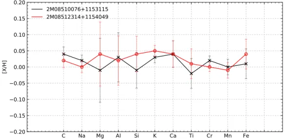
(15) The Astrophysical Journal, 857:14 (19pp), 2018 April 10. Souto et al.. Figure 5. Chemical abundances for the two G-type dwarfs relative to Sun ([X/H], with solar results from this study). The solar abundances ([X/H]=0)±0.05 dex are indicated as dashed lines. This illustrates the close match to a solar abundance pattern (within less than 0.05 dex) of both G dwarfs studied in M67.. The elemental abundances of the two G dwarfs are found to be very consistent with each other, with a mean difference of +0.01±0.03 dex (in the sense of hotter minus cooler star). Figure 5 illustrates the close match to a solar abundance pattern (within less than 0.05 dex) of both solar-like stars in M67. One of the solar-like stars (2M08510076+1153115, or YBP 1514) has an exoplanet detected by Brucalassi et al. (2014, 2016) with a minimum MJup=0.40. The other solar-like star (2M08512314+1154049, or YBP 1587) was reported in Pasquini et al. (2012) to be an exoplanet host candidate. Our derived stellar parameters and metallicity for 2M08510076 +113115 suggest that this star is a solar twin exhibiting abundance differences relative to the Sun of 0.04 dex for all elements. Certain stellar abundance ratios are important for studies of exoplanet properties, such as the C/O ratio, which is one of the factors that affects the ice chemistry in protoplanetary disks (Bond et al. 2010; Teske et al. 2014). Unfortunately, the APOGEE spectra cannot be used to determine precise oxygen abundances in solar-like stars; however, another interesting abundance ratio that affects the interior structure of rocky exoplanets is Mg/Si (Delgado Mena et al. 2010; Brewer & Fischer 2016; and Unterborn & Panero 2017). We derive Mg/Si=0.93 for both M67 G-dwarf stars,22 compared to our same value of 0.93 obtained for the Sun.. the turnoff of the main sequence and the base of the RGB, while 2M08514474+1146460 is near the base of the RGB. Their carbon and nitrogen abundances are found to be slightly different in the two stars, and such differences are expected based on stellar evolution models (e.g., Lagarde et al. 2012): the mean difference (±rms) between both subgiant stars is 0.02±0.04 dex. 5.2.4. Red Clump Stars. The RC stars analyzed here have similar atmospheric parameters: 2M08521856+1144263 with Teff=4842 K, log g=2.45 and 2M08514388+1156425 with Teff=4819 K, log g=2.45. Both stars are members of the RC of M67. As with the other pairs of stellar types isolated here, these M67 RCs share a nearly identical chemistry, with the mean difference in elemental abundances being +0.02±0.03 dex (where the difference is hotter giant—cooler giant). The largest difference is 0.08 dex for 14N, which could be the result of slightly different mixing and mass-loss histories through the FDU and He core flash. 5.3. Signatures of Diffusion in M67 Within the pairs of stars of the same stellar classes analyzed here, the chemical compositions are quite homogeneous, while a comparison across the stellar classes may be used to probe the existence and extent of diffusion. Convective mixing predicts (e.g., Lagarde et al. 2012) that red giant photospheres become richer in nitrogen due to internal stellar nucleosynthesis and deep mixing; however, an increase in the abundances of elements such as Na, Mg, Al, Si, Ca, Mn, and Fe is not expected in lowmass giants, such as those found in M67. Small increases in red giant abundances relative to those of main-sequence and perhaps subgiant stars might be associated with stellar diffusion operating in the hotter main-sequence stars, while the convective envelopes developing in the atmospheres of evolved stars would tend to erase the diffusion signature. As pointed out in Dotter et al. (2017), the atomic diffusion mechanism operates most effectively in the stars’ radiative regions. Önehag et al. (2014) investigated possible diffusion signatures in M67 by studying a sample of hot, mainsequence stars just below the turnoff (Teff∼6130–6200 K), turnoff stars (Teff∼6150–6215 K), and early subgiant stars. 5.2.2. Turnoff Stars. We analyzed two stars from the TOP of the HertzsprungRussell (HR) diagram (2M08514122+1154290: Teff=6119 K, log g=3.91; and 2M08505182+1156559: Teff=6063 K, log g=3.87); the abundances of these two stars have a difference δ=0.07 dex for Mg, K, and Cr, but these are still within the uncertainties in the abundance determinations; see Table 4. 5.2.3. Subgiant Stars. The subgiants analyzed in this work are 2M08513540+1157564 (Teff=5596 K, log g=3.77) and 2M08514474+1146460 (Teff= 5137 K, log g=3.64); 2M08513540+1157564 is located between 22. Mg/Si=N(Mg)/N(Si)=10log N(Mg)/10log N(Si).. 15.
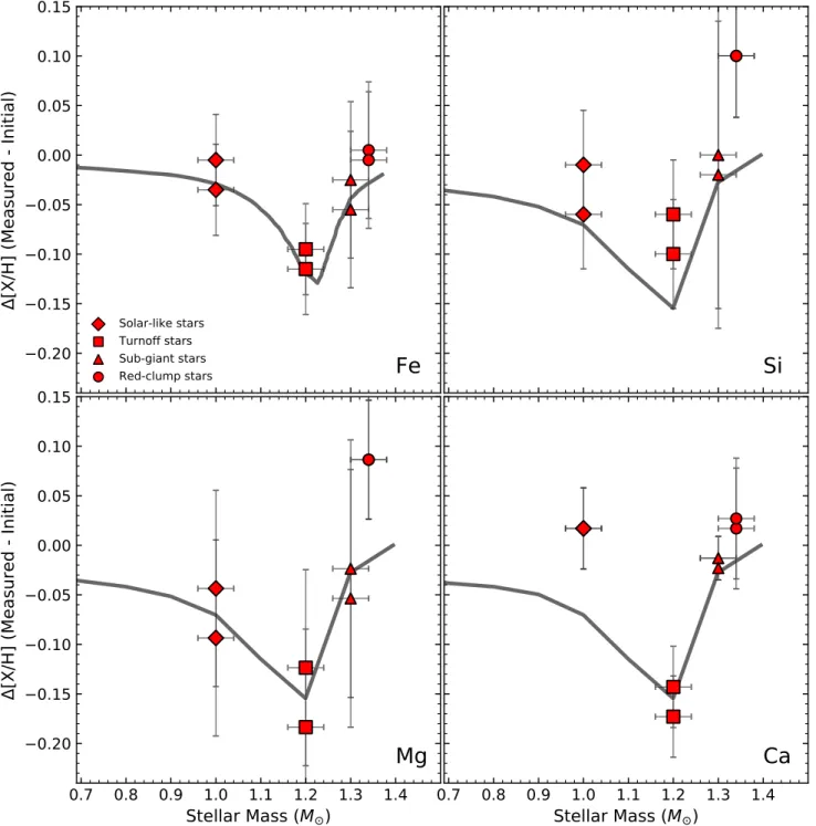
(16) The Astrophysical Journal, 857:14 (19pp), 2018 April 10. Souto et al.. Figure 6. Mean abundances for the red clump (red curve), subgiants (blue curve), and turnoff (green curve) minus abundances for the solar twin 2M08510076 +1153115. The red clump and turnoff stars show systematically higher and lower elemental abundances, respectively, compared to the solar twin.. (Teff∼6040–6110 K). Comparing the abundances in the subgiant and turnoff stars, Önehag et al. (2014) found differences in elemental abundances of Δ(SG–TO)∼+0.02 to +0.06 dex; this is in the correct sense predicted by models of diffusion, as the heavy elements that have sunk below the small convection zones in the hotter turnoff stars are mixed back to the observable surface by the deepening convective envelopes in the subgiants. The specific elements studied by Önehag et al. (2014) were C, O, Na, Al, Si, Mg, S, Ca, Ti, Cr, Mn, Fe, and Ni, and our study includes 10 of these elements in the G dwarfs and subgiants. Results derived here for the turnoff, subgiant, and RC stars compared to those for the solar twin (2M08510076+1153115) are examined to search for the effects of diffusion in M67. Figure 6 plots the differences in the abundances between the turnoff, subgiants, and RCs (their mean abundances for each class) minus the solar twin. The RC stars display larger abundances in most elements relative to the solar twin, which may reflect the convective erasure of a diffusion signature in the solar twin and even more to the turnoff stars, or the pattern may point to systematic effects in the analysis, as the two types of stars have quite different values of effective temperature and surface gravity (see Section 3). The abundance differences in Figure 6 between the subgiants and the solar twin are much smaller in comparison with the RCs, with differences typically <0.05 dex. The stellar parameters between these stars are much more similar than those for the RC stars. The pattern in the differences is interesting and warrants closer examination. The magnitude of diffusion varies from element to element, and Önehag et al. (2014) also indicated in their Figure 8 that the expected magnitude of diffusion is stronger for the individual abundances of warm main-sequence and turnoff stars in M67. From Önehag et al. (2014), the order of the magnitude of the diffusion differences would be expected to be the largest in Na, Mg, Al, Fe, and C, while differences in Mn, Cr, and Si would be smaller and for Ca and Ti almost nonexistent. Examining the subgiant—solar twin pattern, we note that Na, Mg, and Al all exhibit relatively strong positive differences, as do Si, Ca, Mn, and Fe. Interestingly, Ca and Cr show small negative differences. The derived abundances for the turnoff stars set the lower limits for elemental abundances in M67. For almost. all species, we obtain abundance differences <0.10 dex compared to the solar twin, as well as for the other classes. The exceptions were abundances from K, Ti, and Cr, the elements that showed less change in their abundances as a function of log g. Given that there may be small, systematic effects in the absolute abundance scale as derived for the subgiants, turnoff, and solar twin (a few hundredths of a dex), the overall pattern in Figure 6 may indicate that the signature of diffusion in M67 is stronger in turnoff stars, followed by solarlike stars. Figure 6 also indicates that we have an increasing overall metallicity from the turnoff stars to the red clump, with the subgiants and the solar-like stars marginally showing similar levels of chemical composition. When computing overall metallicities for each class (using the [M/H] as the sum of all elemental abundances), we obtain: solar-like stars á [M H]ñ = 0.03 0.05, turnoff stars á [M H]ñ = -0.02 0.00 , subgiants stars á [M H]ñ = 0.02 0.07, and red clump á [M H]ñ = 0.09 0.07, where the uncertainty here represents the standard deviation23 for all elements shown in Figure 6. Recently, Dotter et al. (2017) published predicted surface abundance changes in stellar models that were computed with the MESA code and included atomic diffusion (Paxton et al. 2011, 2013, 2015; see also Choi et al. 2016 and Dotter 2016). Surface abundances of a number of elements were presented for stars in different evolutionary stages (main sequence, turnoff, and RGB), with metallicities varying from −2.0 to 0.0 and ages from 4.0 to 15.0 Gyr. Their results show that both metallicity and age are important factors in the efficacy of atomic diffusion in altering stellar surface abundances. Of particular relevance for this study of M67 are models that were computed for solar metallicity and an age of 4.0 Gyr. Such models are shown as the solid curves in the different panels of Figure 7, which plot Δ[X/H] versus stellar mass, where Δ[X/H]=[X/H]Current−[X/H]Initial for the elements Fe, Mg, Si, and Ca. The filled red symbols represent the elemental abundances derived for the M67 stars, and the pristine Fe abundance for M67 is taken here to be the mean of the K giants, with this value then used as the fiducial point (i.e., δ[Fe/H]=0.00) for the initial cluster value. It should be noted, 23. 16. The uncertainty in the mean is a factor 1/sqrt(2) smaller..
(17) The Astrophysical Journal, 857:14 (19pp), 2018 April 10. Souto et al.. Figure 7. Atomic diffusion models (solar metallicity and 4.0 Gyr; Choi et al. 2016; Dotter et al. 2017) for the stellar mass as a function of Δ[X/H] are shown as the gray lines, where Δ[X/H] indicates the current stellar photospheric abundances of the elements (Fe, Mg, Si, and Ca) minus the initial cluster composition. The filled red symbols represent the elemental abundances derived for the M67 stars.. however, that the abundances of red clump stars are increased due to the reduction of the H budget caused by H burning, but this effect is estimated as being very small (a difference of less than 0.01 dex; Dotter et al. 2017), and that a better initial cluster abundance would be achieved using M-dwarf abundances. (The M dwarfs in M67 would be too faint (H∼15) to be easily observed with APOGEE.) As can be seen from Figure 7, the values of Δ[Fe/H] as a function of stellar mass predicted by the Dotter et al. (2017) models (with [Fe/H]=0.0 and age=4.0 Gyr) exhibit a behavior that is very similar to that found for the M67 stars as a function of their estimated masses. The behavior of the other elements, Ca, Mg, and Si, is reminiscent of that of Fe:. there is a pronounced abundance variation as a function of mass in overall agreement with the atomic diffusion models. However, for Mg and Si, the abundances for the red clump stars are ∼0.10 dex higher than the expectations of the models. In addition, the amplitude of the main-sequence turnoff (MSTO) dip is largest for Ca (given the relatively high Ca abundance in the solar-like stars, which is not in good agreement with the models), while for Mg and Si, the MSTO dip is less pronounced and in better agreement with the models. Elemental abundances derived in the M67 stars covering a range of evolutionary phases suggest that diffusion processes are at work and have been observed in this cluster. Although the number of stars in this initial APOGEE boutique sample is 17.
(18) The Astrophysical Journal, 857:14 (19pp), 2018 April 10. Souto et al.. Foundation (NSF) under grants AST-1311835 and AST1715662. S.V. gratefully acknowledges the support provided by Fondecyt reg. no. 1170518. H.J. acknowledges support from the Crafoord Foundation and Stiftelsen Olle Engkvist Byggmästare. Funding for the Sloan Digital Sky Survey IV has been provided by the Alfred P. Sloan Foundation, the US Department of Energy Office of Science, and the Participating Institutions. SDSS-IV acknowledges support and resources from the Center for High-Performance Computing at the University of Utah. The SDSS website is www.sdss.org. SDSS-IV is managed by the Astrophysical Research Consortium for the Participating Institutions of the SDSS Collaboration, including the Brazilian Participation Group, the Carnegie Institution for Science, Carnegie Mellon University, the Chilean Participation Group, the French Participation Group, the HarvardSmithsonian Center for Astrophysics, Instituto de Astrofísica de Canarias, the Johns Hopkins University, the Kavli Institute for the Physics and Mathematics of the Universe (IPMU)/University of Tokyo, Lawrence Berkeley National Laboratory, Leibniz Institut für Astrophysik Potsdam (AIP), Max-Planck-Institut für Astronomie (MPIA Heidelberg), Max-Planck-Institut für Astrophysik (MPA Garching), Max-Planck-Institut für Extraterrestrische Physik (MPE), the National Astronomical Observatory of China, New Mexico State University, New York University, the University of Notre Dame, Observatório Nacional/MCTI, the Ohio State University, Pennsylvania State University, the Shanghai Astronomical Observatory, the United Kingdom Participation Group, Universidad Nacional Autónoma de México, the University of Arizona, the University of Colorado Boulder, the University of Oxford, the University of Portsmouth, the University of Utah, the University of Virginia, the University of Washington, the University of Wisconsin, Vanderbilt University, and Yale University. Facility: Sloan. Software: Turbospectrum (Plez 2012), (Alvarez & Plez 1998), Numpy (Van Der Walt et al. 2011), Matplotlib (Hunter 2007).. small, the comparison of spectroscopically derived Fe abundances with those predicted by stellar models that include atomic diffusion is very promising, and this pilot study demonstrates what can be accomplished with the APOGEE spectra. D. Souto et al. (2018, in preparation) will present abundances for a much larger sample of M67 members based on the stellar parameters obtained from photometry and isochrones and chemical abundances derived automatically from the APOGEE spectra; these results will also be compared with the DR14 abundances. 6. Summary This paper presents detailed chemical abundances for the elements C, N, O, Na, Mg, Al, Si, K, Ca, Ti, V, Cr, Mn, and Fe in eight stellar members of the open cluster M67. The sample stars have different stellar masses and are in different evolutionary stages: two G dwarfs, two turnoff stars, two G subgiants, and two K giants (RC). Abundances were derived via a manual “boutique” detailed spectroscopic line-by-line abundance analysis using APOGEE high-resolution NIR spectra. The derived abundances were investigated as a function of stellar evolutionary state, with homogeneous abundances found for each pair of stars in the same phase of evolution. Significant changes in abundance (∼0.05–0.20 dex) were found across different evolutionary states, with most of the studied elements (except K, Ti, and Cr) having their lowest values in the turnoff stars, while the RC stars tended to exhibit the largest abundances. For iron, in particular, we obtain áA (Fe)ñ = 7.48 0.05 for solar-like stars, áA (Fe)ñ = 7.39 0.05 for turnoff stars, áA (Fe)ñ = 7.46 0.08 for subgiant stars, and áA (Fe)ñ = 7.50 0.07 for RC stars. We have conducted a comparison of the derived abundances of Mg, Si, Ca, and Fe as a function of stellar mass with atomic diffusion models in the literature (Choi et al. 2016; Dotter 2016; Dotter et al. 2017). We find that the atomic diffusion models explain reasonably well most of the observed abundance trends, suggesting that the signature of diffusion has been detected in M67 stars. Published departures from LTE-derived abundances from Na I, Mg I, and Si I lines in the APOGEE spectral region were examined and are expected to be significantly smaller than the changes in abundance found in the M67 stars: non-LTE is unlikely to explain the observed abundance spreads that correlate with evolutionary state, but 3D calculations are still needed. Diffusion effects will be investigated further using the entire set of APOGEE spectra and ASPCAP results for M67 members in a follow-up paper.. ORCID iDs Diogo Souto https://orcid.org/0000-0002-7883-5425 C. Allende Prieto https://orcid.org/0000-0002-0084-572X D. A. García-Hernández https://orcid.org/0000-00021693-2721 Marc Pinsonneault https://orcid.org/0000-0002-7549-7766 Peter Frinchaboy https://orcid.org/0000-0002-0740-8346 Jon Holtzman https://orcid.org/0000-0002-9771-9622 J. A. Johnson https://orcid.org/0000-0001-7258-1834 Henrik Jönsson https://orcid.org/0000-0002-4912-8609 Steven R. Majewski https://orcid.org/0000-00032025-3147 Matthew Shetrone https://orcid.org/0000-0003-0509-2656 Guy Stringfellow https://orcid.org/0000-0003-1479-3059 Ricardo Carrera https://orcid.org/0000-0001-6143-8151 Keivan Stassun https://orcid.org/0000-0002-3481-9052 Dante Minniti https://orcid.org/0000-0002-7064-099X Felipe Santana https://orcid.org/0000-0002-4023-7649. We thank the anonymous referee for useful comments that helped improve the paper. We thank Jo Bovy and Dennis Stello for useful comments. K.C. thanks Corinne Charbonnel for fruitful conversations and Karin Lind for checking non-LTE corrections for Na. K.C. and V.S. acknowledge that their work here is supported in part by the National Aeronautics and Space Administration under grant 16-XRP16_2-0004, issued through the Astrophysics Division of the Science Mission Directorate. D.A.G.H. was funded by Ramón y Cajal fellowship number RYC-2013-14182. D.A.G.H. and O.Z. acknowledge support provided by the Spanish Ministry of Economy and Competitiveness (MINECO) under grant AYA-2014-58082-P. P.M.F. acknowledges support provided by the National Science. References Alvarez, R., & Plez, B. 1998, A&A, 330, 1109 Andrievsky, S. M., Spite, M., Korotin, S. A., et al. 2008, A&A, 481, 481 Asplund, M. 2005, ARA&A, 43, 481 Asplund, M., Grevesse, N., Sauval, A. J., & Scott, P. 2009, ARA&A, 47, 481. 18.
(19) The Astrophysical Journal, 857:14 (19pp), 2018 April 10. Souto et al.. Bergemann, M., Lind, K., Collet, R., Magic, Z., & Asplund, M. 2012, MNRAS, 427, 27 Bertelli Motta, C., Salaris, M., Pasquali, A., & Grebel, E. K. 2017, MNRAS, 466, 2161 Blanco-Cuaresma, S., Soubiran, C., Heiter, U., et al. 2015, A&A, 577, A47 Blanton, M. R., Bershady, M. A., Abolfathi, B., et al. 2017, AJ, 154, 28 Bond, J. C., O’Brien, D. P., & Lauretta, D. S. 2010, ApJ, 715, 1050 Bovy, J. 2016, ApJ, 817, 49 Bressan, A., Marigo, P., Girardi, L., et al. 2012, MNRAS, 427, 127 Brewer, J. M., & Fischer, D. A. 2016, ApJ, 831, 20 Brucalassi, A., Pasquini, L., Saglia, R., et al. 2014, A&A, 561, L9 Brucalassi, A., Pasquini, L., Saglia, R., et al. 2016, A&A, 592, L1 Carpenter, J. M. 2001, AJ, 121, 2851 Casamiquela, L., Carrera, R., Blanco-Cuaresma, S., et al. 2017, MNRAS, 470, 4363 Choi, J., Dotter, A., Conroy, C., et al. 2016, ApJ, 823, 102 Cohen, J. G. 1980, ApJ, 241, 981 Cunha, K., Smith, V. V., Johnson, J. A., et al. 2015, ApJL, 798, L41 Delgado Mena, E., Israelian, G., González Hernández, J. I., et al. 2010, ApJ, 725, 2349 Dotter, A. 2016, ApJS, 222, 8 Dotter, A., Conroy, C., Cargile, P., & Asplund, M. 2017, ApJ, 840, 99 Foy, R., & Proust, D. 1981, A&A, 99, 221 Friel, E. D., & Boesgaard, A. M. 1992, ApJ, 387, 170 Friel, E. D., Jacobson, H. R., & Pilachowski, C. A. 2010, AJ, 139, 1942 García Pérez, A. E., Allende Prieto, C., Holtzman, J. A., et al. 2016, AJ, 151, 144 Geller, A. M., Latham, D. W., & Mathieu, R. D. 2015, AJ, 150, 97 Gonzalez, G. 2016, MNRAS, 459, 1060 González-Hernández, J. I., & Bonifacio, P. 2009, A&A, 497, 497 Gunn, J. E., Siegmund, W. A., Mannery, E. J., et al. 2006, AJ, 131, 2332 Gustafsson, B., Edvardsson, B., Eriksson, K., et al. 2008, A&A, 486, 951 Holtzman, J. A., Shetrone, M., Johnson, J. A., et al. 2015, AJ, 150, 148 Hunter, J. D. 2007, CSE, 9, 90 Jacobson, H. R., Pilachowski, C. A., & Friel, E. D. 2011, AJ, 142, 59 Korn, A. J., Grundahl, F., Richard, O., et al. 2007, ApJ, 671, 402 Lagarde, N., Decressin, T., Charbonnel, C., et al. 2012, A&A, 543, A108 Leiner, E., Mathieu, R. D., Stello, D., Vanderburg, A., & Sandquist, E. 2016, ApJL, 832, L13 Lind, K., Asplund, M., Barklem, P. S., & Belyaev, A. K. 2011, A&A, 528, A103 Lind, K., Korn, A. J., Barklem, P. S., & Grundahl, F. 2008, A&A, 490, 777 Liu, F., Asplund, M., Yong, D., et al. 2016, MNRAS, 463, 696 Majewski, S. R., Schiavon, R. P., Frinchaboy, P. M., et al. 2017, AJ, 154, 94. Michaud, G., Alecian, G., & Richer, J. 2015, Atomic Diffusion in Stars (Switzerland: Springer International Publishing) Michaud, G., Richard, O., Richer, J., & VandenBerg, D. A. 2004, ApJ, 606, 452 Montegriffo, P., Ferraro, F. R., Origlia, L., & Fusi Pecci, F. 1998, MNRAS, 297, 872 Nidever, D. L., Holtzman, J. A., Allende Prieto, C., et al. 2015, AJ, 150, 173 Nordlander, T., Korn, A. J., Richard, O., & Lind, K. 2012, ApJ, 753, 48 Önehag, A., Gustafsson, B., & Korn, A. 2014, A&A, 562, A102 Osorio, Y., & Barklem, P. S. 2016, A&A, 586, A120 Pancino, E., Carrera, R., Rossetti, E., & Gallart, C. 2010, A&A, 511, A56 Pasquini, L., Brucalassi, A., Ruiz, M. T., et al. 2012, A&A, 545, A139 Paxton, B., Bildsten, L., Dotter, A., et al. 2011, ApJS, 192, 3 Paxton, B., Cantiello, M., Arras, P., et al. 2013, ApJS, 208, 4 Paxton, B., Marchant, P., Schwab, J., et al. 2015, ApJS, 220, 15 Plez, B. 2012, Turbospectrum: Code for Spectral Synthesis, Astrophysics Source Code Library, ascl:1205.004 Price-Jones, N., & Bovy, J. 2018, MNRAS, 475, 1410 Prša, A., Harmanec, P., Torres, G., et al. 2016, AJ, 152, 41 Salaris, M., Weiss, A., & Percival, S. M. 2004, A&A, 414, 163 Sarajedini, A., Mancone, C. L., Lauer, T. R., et al. 2009, AJ, 138, 184 Schlegel, D. J., Finkbeiner, D. P., & Davis, M. 1998, ApJ, 500, 525 Shetrone, M., Bizyaev, D., Lawler, J. E., et al. 2015, ApJS, 221, 24 Skrutskie, M. F., Cutri, R. M., Stiening, R., et al. 2006, AJ, 131, 1163 Smiljanic, R., Romano, D., Bragaglia, A., et al. 2016, A&A, 589, A115 Smith, V. V., Cunha, K., Shetrone, M. D., et al. 2013, ApJ, 765, 16 Souto, D., Cunha, K., García-Hernández, D. A., et al. 2017, ApJ, 835, 239 Souto, D., Cunha, K., Smith, V., et al. 2016, ApJ, 830, 35 Stello, D., Vanderburg, A., Casagrande, L., et al. 2016, ApJ, 832, 133 Tautvaišiene, G., Edvardsson, B., Tuominen, I., & Ilyin, I. 2000, A&A, 360, 499 Taylor, B. J. 2007, AJ, 134, 934 Teske, J. K., Cunha, K., Smith, V. V., Schuler, S. C., & Griffith, C. A. 2014, ApJ, 788, 39 Unterborn, C. T., & Panero, W. R. 2017, ApJ, 845, 61 Van Der Walt, S., Colbert, S. C., & Varoquaux, G. 2011, arXiv:1102.1523 Wilson, J. C., Hearty, F., Skrutskie, M. F., et al. 2010, Proc. SPIE, 7735, 77351C Yadav, R. K. S., Bedin, L. R., Piotto, G., et al. 2008, A&A, 484, 609 Yong, D., Carney, B. W., & Teixera de Almeida, M. L. 2005, AJ, 130, 597 Zasowski, G., Johnson, J. A., Frinchaboy, P. M., et al. 2013, AJ, 146, 81 Zhang, J., Shi, J., Pan, K., Allende Prieto, C., & Liu, C. 2016, ApJ, 833, 137 Zhang, J., Shi, J., Pan, K., Allende Prieto, C., & Liu, C. 2017, ApJ, 835, 90. 19.
(20)
Figure


+7


Documento similar
