TítuloHousehold Debt and Consumption Inequality: The Spanish Case

Texto completo

(1)Economies 2014, 2, 147-170; doi:10.3390/economies2030147 OPEN ACCESS. economies ISSN 2227-7099 www.mdpi.com/journal/economies Article. Household Debt and Consumption Inequality: The Spanish Case Gonzalo Paz Pardo 1,† and José Manuel Sánchez Santos 2,†,* 1. 2. †. University College London, Gower St, London WC1E 6BT, UK; E-Mail: gonzalo.pardo.13@ucl.ac.uk Faculty of Economics, Universidade da Coruña, Campus de Elviña, s/n, 15071 A Coruña, Spain These authors contributed equally to this work.. * Author to whom correspondence should be addressed; E-Mail: jose.manuel.sanchez@udc.es; Tel.: +34-981-167-000 (ext. 2584); Fax: +34-981-167-070. Received: 29 November 2013; in revised form: 4 July 2014 / Accepted: 9 July 2014 / Published: 21 July 2014. Abstract: The aim of this paper is twofold. On the one hand, we attempt to find out whether Spanish households took part in a process of substituting loans for wages during the period before the beginning of the current economic crisis. On the other hand, we try to identify the consequences of such process in the evolution of income and consumption inequalities. The theoretical framework to deal with the above mentioned issues is provided by a review of the economic literature on the determinants of consumer behaviour, namely, on consumption, saving and debt. The empirical study consists of a descriptive analysis, which is focused on two fields. First, we analyze the evolution of consumer credit (both, in aggregate and by income groups) and the savings rates. Second, we compare the values and temporal evolution of income and consumption inequalities. The period under study ranges from 2000 to 2008. Our analysis provides some empirical evidence that supports the hypothesis that financial conditions led to significant effects on the distribution of consumption. This influence is especially significant in the case of consumption inequalities. These inequalities were lower than income inequalities and were kept “artificially” low and stable during the whole period. Keywords: financial conditions; household indebtedness; consumer credit; income distribution; consumption inequalities.

(2) Economies 2014, 2. 148. 1. Introduction The positive macroeconomic effects of a developed and efficient financial system have been well documented in economic literature. For example, King and Levine [1] established a very close correlation between the development of the financial sector in an economy and variables like economic growth, capital accumulation and improvements in the efficiency of the use of physical capital. However, the role of the financial system can also be addressed from the perspective of its relationship to the inequalities in the distribution both of income and consumption. The evolution of inequalities and the causes that explain them are topics with a notable presence in the economic research agenda, yet far fewer studies have attempted to explore the link of this variable with financial conditions. A priori, a financial system that operates properly, in particular, if financial institutions properly value risk and there are no adverse shocks, could facilitate wide access to credit, allowing individuals to optimize the distribution of their expected income throughout their lives. Under these circumstances, this optimization process does not necessarily have negative macroeconomic consequences. Furthermore, the ease of access could favour the reduction of inequalities, especially those which are established in terms of consumption. This latter kind of influence is consistent with the results of Heathcote, Perri and Violante [2] and Agnello and Sousa [3]. In the first case, the authors provide evidence that access to the financial markets has reduced both the magnitude and the growth of consumption inequalities in terms of consumption in the United States since the 1980s. For their part, Agnello and Sousa [3], based on a panel of 62 countries, conclude that better access to credit also reduced inequalities. In a similar vein, Barba and Pivetti [4] argue that developments in financial sector development allowed households to meet with loans the demand that they were not able to meet with their wages. This is what these authors call a substitution of debt (loans) for wages. As a consequence of this process, households indebtedness increased sharply, giving rise to concerns about the sustainability of this debt. In a similar line, Rajan [5] argues that in the United States the increase in inequalities was “hidden” by credit expansion. These inequalities were derived mainly from differences in education, but also from other causes (the process of deregulation, the influx of immigrants, tax cuts for the richest, a minimum wage barely growing, etc.). According to this author, with the aim of preventing such an increase in inequalities becoming a social problem, the US authorities supported loans to households with an increasingly lower income, mainly for the purchase of housing. In this way, “inequality was hidden”, households felt wealthier and consumption increased. More recently, Galbraith [6] provides a more detailed analysis about this rise in inequality. This author finds that there are common global patterns in economic inequality across different countries that appear to be very strongly related to major events affecting the world economy as a whole. Particularly, the most important have been changes in financial regimes and changes in systems of financial governance. In his own words: “The economics of inequality is, in large measure, an economics of instability; inequality is the barometer, in many ways, of the instabilities that global credit relationships create” (Galbraith, [6], p. 18)..

(3) Economies 2014, 2. 149. The private sector’s debt and, in particular, households’ indebtedness have substantial macroeconomic implications. The important role played by this variable both in the expansionary (before 2008) and recessive phase (from 2008 onwards) of the last business cycle in numerous developed economies has placed households’ indebtedness at the centre of the debate regarding the recent financial crisis. In particular, a special emphasis is placed on the role played by high levels of household leverage as a factor influencing the possibilities and the rhythm of the economy recovering in several developed economies after the last recession. In addition, some authors have highlighted that one of the consequences of the increase in households’ indebtedness is that they become much more sensitive to changes that might occur in macroeconomic conditions such as a rise in unemployment, increases in interest rates or a fall in the housing price (Debelle, [7]). According to these kinds of considerations and taking into account that in the economic literature few studies have attempted to explore the implications in terms of inequality of the evolution of households’ indebtedness, the main objective of this study is to verify the hypothesis that in the last expansionary phase of the business cycle in the Spanish economy, the increase in household consumption levels was financed mainly through the recourse to borrowing that, in turn, favoured the reduction of inequalities, particularly in terms of consumption. In this context, the main contribution of this work is to deal with the link between household indebtedness and the evolution of inequalities in Spain since 2000. In principle, this link may have a two-way nature: the evolution of inequalities can act as a determinant of borrowing and, at the same time, rising household debt levels may have distributional consequences for income and consumption.1 Most of the research on inequalities in Spain is unanimous in identifying higher levels of unemployment as the main variable determining factor causing an increase in inequality. Other variables that appear in the literature are the level of GDP, public spending and transfers in the public sector, higher education and inflation. 2 In this context, the issue addressed in this work is novel because as far as we know regarding the Spanish case, there is no research on the relationship between financial conditions (deregulation, monetary policy, cost, funding, etc.) and economic inequalities. This shortcoming gives our analysis a special interest, to the extent that knowledge of the distributional implications that may arise from the financial conditions is relevant to inform policy decisions. This paper is organized as follows: Section 2 reviews some of the explanatory hypotheses of the consumer behaviour explaining borrowing and, particularly, consumer demand of credit. Section 3 deals with the evolution of the households’ indebtedness and real wage levels in Spain. Section 4 analyses the link between the evolution of households’ indebtedness and the degree of income and consumption inequalities. In Section 5, some empirical evidence is provided. Finally, Section 6 draws the main conclusions.. 1. The source of data on which this study is based is the Encuesta Financiera de las Familias (Survey of Household Finance) (EFF), a triennial survey developed by the Bank of Spain since 2002 [8]. There are EFF for 2002, 2005 and 2008 [8]. Currently is under development and publication the EFF for the year 2011. 2 For detailed studies on this topic, see Pijoan-Mas and Sánchez Marcos [9], Farré and Vella [10], Hospido and Bonhomme [11], Ayala, Canto and Rodriguez [12] and Addabo, García-Fernández, Rodríguez-Llorca and Maccagnan [13]. The Informe sobre la Desigualdad en España [14], published by Fundación Alternativas includes a series of works related to the problems of income distribution and inequality in Spanish society..

(4) Economies 2014, 2. 150. 2. Analytical Framework 2.1. Determinants of Consumption and Borrowing Decisions: Beyond the Conventional Explanations According to the traditional Keynesian formulation of consumption function, the consumption of an individual in a period basically depends on the disposable income in the same period. However, individuals can distribute their consumption throughout their life in the manner they consider appropriate and regardless of their current income, through the use of borrowing (current consumption at the expense of future income) and saving (future consumption at the expense of current income). Following this line, one of the traditional explanations to the households’ indebtedness of families has its roots in the theories of the permanent income (Friedman, [15]) and “life cycle” (Ando and Modligliani, [16]; and Modigliani, [17]). However, when it comes to delving into the causes that explain household behaviour, it is important to explore the role of some factors that can lead individuals to consuming and borrowing, outside or above the levels predicted by the hypothesis of permanent life-income cycle. In order to carry out this type of analysis, it is necessary to go far beyond the assumption of a fully rational consumer in the most orthodox sense of the term. In particular, this type of approach is essential to elucidate whether the existence of a process of substitution of debt for wages is a consumer behaviour that strictly meets the criterion of the maximization of an intertemporal utility function or, by contrast, is explained by other type of reasons. Authors such as Foster and Magdoff [18], who adopt a more heterodox view, point out that, in the U.S. economy, individuals rely on borrowing as a means of maintaining their standard of living in a context of wage stagnation (or as “desperate” means of increasing their standard of living). According to their approach, it could be argued to some extent that in the late 1990s U.S. economic expansion was “bought” with debt, especially household debt that is mainly related to housing, and to low income households. In the same line, Foster [19] argues that this type of reasoning can be extrapolated to the period 2000–2006 and potentially with many more devastating consequences. In the context of a model that seeks to explain the effects of income distribution on consumption expenditure, Brown [20] concluded that broader access to credit allowed an increase in the purchasing power of middle-low income groups. Therefore, the removal of the so-called “income constraint” allows consumption and the propensity to consume in individuals by these income groups to increase. Although inequality increases, its potential effect on consumption may be mitigated by the expansion of consumer credit. In this sense, this author warns that U.S. growth dangerously relied on the willingness of a significant segment of the population to borrow at a level that, eventually, could cause them serious financial pressures. Iacoviello [21] develops a model that attempts to explain the evolution of indebtedness and the degree of wealth and consumption inequalities. The results of this analysis showed that although the changes in the economic cycle affect household indebtedness, the substantial growth of this variable in the United States can only be explained by taking into account the increasing degree of inequality in the income distribution. According to this author, the growth of inequalities in wealth and the slight increasing trend (far less than income inequalities) of consumption inequality can be explained with his model based on the income distribution..

(5) Economies 2014, 2. 151. Taking the American case as a reference, Barba and Pivetti [4] argue that the tensions that led individuals to consume “beyond their means” are related to the slow growth of real incomes, the attractiveness of new consumer goods (related to new technologies, etc.) and the desire to emulate individuals with higher incomes. In a later work, these same authors reiterate that the factors most commonly cited as determinants of the last economic and financial crisis (low rates of interest, global imbalances, etc.) are not the real causes. On the contrary, the crucial point was an economic scenario characterized by stagnant wages and growing economic inequalities. Under these circumstances, low interest rates fostered the growth of households’ indebtedness and, furthermore, economic authorities tried to replace this private debt with public debt, so as to maintain the stability of the financial system (Barba and Pivetti, [22]).3 These points are further illustrated in Rancière and Kumhof [24]. These authors provide a theoretical framework for explaining the connection between inequality, leverage and financial crises. Their model shows how rising inequality in a climate of rising consumption can lead poorer households to increase their leverage. Particularly, according to these authors’ model, an increase in the bargaining power of high income households causes them to have higher incomes, which are given back to the rest of the population via loans. This situation allows lower-income households to maintain their consumption levels, but eventually leads to higher leverage and to a higher probability of a financial crisis. 2.2. Liquidity Constraints Previous explanations based on permanent income-life cycle models and on the desires of individuals to access borrowing from other causes do not always adequately match the reality. Any individual can save whenever he/she so wishes, but not any individual can borrow, because access to borrowing is subject to someone’s willingness to lend the funds. It is common for individuals to confront the so-called liquidity constraints (either in terms of the amount they can borrow or the interest rate to be paid), which prevent the theoretical assumptions from being carried out in practice (Shapiro, [25]). In this area, Campbell and Mankiw [26] argue that consumption is better explained by dividing consumers into two categories: on the one hand, individuals who consume on the basis of their current income and, on the other hand, individuals who consume according to their permanent income. These groups therefore correspond with those who are facing financial restrictions and those that do not, respectively. From this, it is clear that the existence of restrictions that limit the capacity of certain consumers to freely distribute their consumption over time will be determined by the financial conditions. If for any reason, their credit conditions are particularly favourable, the above mentioned liquidity constraints are reduced and consumption tends to increase (Bacchetta and Gerlach, [27]). In addition, it should be noted that the expansion of the supply of credit not only affects the total volume of consumption, but also its distribution. As credit conditions improve, the credit becomes increasingly available for households with a lower level of income or wealth, which were previously subject to “liquidity constraints”. 3. More recently, Barba and Pivetti [23] even argue that the trend towards austerity prevailing today in Europe could be understood, in a way, as a continuation of that process of substitution of debt for wages..

(6) Economies 2014, 2. 152. In this sense, there are numerous studies showing the positive effects that financial deregulation and innovation has had (since the 1980s) in terms of relaxing these restrictions on liquidity. In particular, one of these effects is a rise in the level of consumption that households can access because they are less limited when it comes to borrowing against their future income (Boone, Girouard and Wanner, [28]; Brady, [29]; Brady, [30] and Aron et al. [31]). In regard to financial innovation, Brown [32] argues that the expansion of financial engineering (particularly after 1987) played an important role in making consumer credit more widely available and it was crucial for the growth of consumption in the U.S. In light of the above considerations and insofar as that an expansive monetary policy in general involves more favourable financial conditions, it can be expected that monetary policy also has effects on both levels of consumption and its distribution. By the end of the 1990s, Galbraith [33] pointed out that the growth of inequality in the United States was related to the poor performance of the American economy which, in turn, was the result of inadequate policies, in particular, the interest rates set by the Federal Reserve. In fact, as regards the redistributive role of the monetary policy, Coibion et al. [34] provide some evidence that restrictive monetary policy causes long term increases in inequalities across households (in terms of whole income, labour income, consumption or total expenditure), clarifying that such effects are particularly visible in consumption inequalities. Finally, it should be noted that a factor that can significantly influence the liquidity constraints is the “wealth effect”, which refers to the increase in consumption linked to the rise in the price of financial and real assets. Economic literature dealing with the relationship between asset prices and consumption is profuse.4 Among the arguments put forward, the most relevant one for the purposes of our analysis is that the increase in the price of the assets allows individuals a growing access to credit. This is a way of relaxing the financial constraints faced by households with low levels of income or wealth (Bernanke and Gertler [38]). In countries like the United Kingdom or the United States, the Mortgage Equity Withdrawal (MEW) has become a widespread financial practice, a financial transaction which consists of getting a mortgage extension by using the increase in housing value. One of the factors that led to the expansion of this practice was the favourable fiscal treatment that it gets, for example, in the U.S. In the Spanish case, it can be expected that the wealth effect is especially relevant given the well-known fact that it is one of the European countries with the highest homeownership rates (82.2% according to INE data). Insofar as the liquidity restrictions primarily affect individuals with low levels of income and wealth, the favourable financial conditions that contribute to lifting these restrictions, will have redistributive effects. These effects can be explained because more individuals will be able to distribute their consumption as they wish by means of borrowing. In short, under these conditions, the number of individuals subject to liquidity constraints is reduced and individuals of lower income (and wealth) can increasingly access borrowing, which will favour the reduction of inequalities in terms of consumption. 4. As an example can be mentioned Pichette and Tremblay [35], Carroll, Otsuka and Slacalek [36] and Case, Quigley and Shiller [37]. These authors also estimate the wealth effect, trying to discern if the effect associated with financial assets is greater or less than the real assets one..

(7) Economies 2014, 2. 153. If this argument is integrated into the above mentioned theories of consumption, if an individual is not restricted to liquidity constraints, he/she can distribute his/her consumption according to the predictions derived from the theories of the permanent life-income cycle. The individual can also, if this is the case, use the debt to try to access higher levels of consumption in comparison with other individuals or access new emergent products. Therefore, via both routes, it seems likely that an individual who is no longer subject to liquidity constraints will increase his/her consumption. Within the framework of this approach, the objective of this work is to analyze, first, to what extent liquidity constraints were eased in Spain over the period starting at the beginning of the 2000s and, second, the distributional consequences that this may have. This is a matter of special relevance, given that, contrary to what was happening in the expansionary phase of the business cycle, the recent financial turmoil gives rise to a scenario of restrictive financial conditions. In particular, access to credit has been made extremely difficult and, according to the above formulated hypothesis, a growth of inequality, especially in terms of consumption, could be expected. 3. Household Debt and Wages in Spain 3.1. Households Indebtedness: Components and Evolution One of the indicators that reveal the magnitude of households’ indebtedness in Spain is the ratio volume of loans to disposable income. For purposes of assessing to what extent households borrow so as to finance their consumption, the total debt is divided into two main segments: mortgage debt (in the Spanish case they represent the greatest part of households debt), and non-mortgage debt (consisting of credits and loans to households and other non-mortgage debts. Within this last category, those of greater importance are consumer loans, although, for example, loans and credits for the purchase of securities or other purposes are also included. Moreover, this category can also include some loans not classified as “home loans”, but in practice intended for housing. Despite these nuances, in the follow-up, we use this variable as a “proxy” of the funding intended for consumption. In the Spanish case, the continuous and significant growth of the ratios of both types of debt to households’ gross disposable income over the period 2000–2007 is evident (Figure 1)..

(8) Economies 2014, 2. 154. Figure 1. Households and Non Profit Institutions Serving Households (NPISH) debt-to-income ratio. % annual household Gross Disposable Income (GDI). 140 120. Housing‐related. Other. 100 80 60 40 20 0. Source: own ellaboration with data from Banco de Espana (BdE) and Instituto Nacional de Estadistica (INE).. During this period, not only did mortgage debt grow, but the rest of household debt also experienced a sharp expansion (Figure 2). Figure 2. Consumer debt for households and NPISHs.. % household GDI (4 previous quarters). 36 34 32 30 28 26 24 22 20. Source: own ellaboration with data from BdE and INE. Shaded areas indicate recessions.. The above mentioned time path of this variable may be associated with a context of increasing credit demand as well as highly flexible supply of credit conditions (reduction of the liquidity constraints). In particular, the total volume of non-mortgage debt increased from 24.57% of the households RDB by the end of the year 2000 to 34.13% in the second quarter of 2008. This growth should also be.

(9) Economies 2014, 2. 155. viewed within the perspective of a context of significant increase in the RDB of households (in some years exceeding annual growth rates of 6% in nominal terms). Furthermore, it is interesting to note that this variable has been declining slowly and irregularly since 2008. The evolution of the credits officially classified by financial institutions as “credit for consumer durables” (an important part of the credits for consumption) in terms of RDB is represented in Figure 3. The evolution of this variable, despite being more irregular, is similar to the previous one. The values are significant and grew until the beginning of 2008, the moment when they collapsed. This crash can be linked to a progressive comeback of restrictions on liquidity as a result of the crisis that affected the European and, particularly, Spanish financial sector. Figure 3. Volume of credit for durable consumption.. % household GDI (last 4 quarters). 9 8.5 8 7.5 7 6.5 6 5.5 5 4.5. Source: own ellaboration with data from BdE and INE. Shaded areas indicate recessions.. The time path of real rates of growth of non-mortgage debt, which we identify with the consumer credit (FINC), presents important similarities with the evolution of consumption (C). The evolution of these variables along with the relative importance of the consumer credit regarding household consumption (FINCF/C) is reflected in Figure 4. This evidence suggests that the tendency of consumer credit growth predicts the evolution of consumption.5. 5. This observation is in line with the results of authors like Antzoulatos [39] and Ludvigson [40]..

(10) Economies 2014, 2. 156 Figure 4. Consumption and consumer credit.. 15. 10. %. 5. 0. ‐5. ‐10. ‐15 Consumer credit/Consumption. Growth of consumption. Growth of consumer credit. Source: own ellaboration with data from Bank of Spain (BdE), Spanish National Statistics Institute (INE) and Organization for Economic Cooperation and Development (OECD). Growth rates are real and expressed in interannual terms. The ratio consumer credit/consumption is a SMA for the previous 4 quarters. Shaded areas indicate recessions.. 3.2. Credit Supply Conditions As stated in the theoretical argumentation, credit supply conditions play a role in easing the “liquidity constraints” for certain households and, thus, in allowing them to raise their indebtedness. Credit supply conditions consist of numerous elements, many of which are hard to extract from statistic data. Nevertheless, for illustrative purposes, we chose real interest rates as a representative variable of the credit supply environment. During the period under study, and mostly because Spain joined the EMU, real interest rates for consumer credit remained at historically low values (Figure 5): credit supply conditions were undoubtedly favorable during the pre-crisis years. Nevertheless, it should not be ignored that a housing loan is also a way of substituting loans for wages, and that the growth of housing loans was spectacular in Spain between 2000 and 2008 (in terms of disposable income). This kind of consideration could be a first indication that families were actually resorting to borrowing to supplement their current incomes, thus supporting the application of Barba and Pivetti’s [4] hypothesis in Spain..

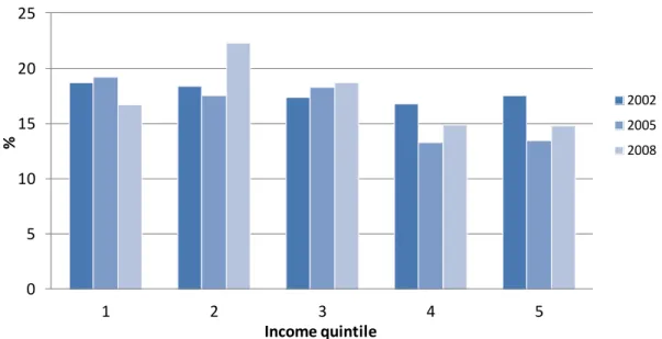
(11) Economies 2014, 2. 157 Figure 5. Real interest rates for credit consumption.. 16.00. Real interest rates. 14.00 12.00 10.00 8.00 6.00 4.00 2.00. JUL 1991 FEB 1992 SEP 1992 APR 1993 NOV 1993 JUN 1994 JAN 1995 AUG 1995 MAR 1996 OCT 1996 MAY 1997 DEC 1997 JUL 1998 FEB 1999 SEP 1999 APR 2000 NOV 2000 JUN 2001 JAN 2002 AUG 2002 MAR 2003 OCT 2003 MAY 2004 DEC 2004 JUL 2005 FEB 2006 SEP 2006 APR 2007 NOV 2007 JUN 2008 JAN 2009 AUG 2009 MAR 2010 OCT 2010 MAY 2011 DEC 2011. 0.00. Banks. Savings banks. Source: own ellaboration with data from BdE and INE.. 3.3. Debt by Income Groups The analysis of the distribution of debt by income groups is relevant, since we would not be talking about a leveling effect of credit if the distribution of the aforementioned indebtedness corresponded basically to higher income individuals. As the Survey of Household Finances (EFF) provides information about households’ income, we can break down this analysis by income groups. First, with regards to liquidity constraints, it is clear from Figure 6 that the lowest income quintile is very liquidity-constrained. For the entire period, over 40% of families in this income quintile who applied for a loan were rejected or given a smaller amount (we also include in this percentage those families who did not apply for a loan because they felt that their application would be rejected). Of course, following the basic logic, liquidity constraints decrease as income increases. It is also relevant to note the substantial increase in overall liquidity constraints that took place in 2008. With regard to the percentage of individuals who have outstanding debts, the data in Table 1 are consistent with the earlier analysis for liquidity constraints. On the one hand, the table shows that households in the first income quintile are liquidity constrained. Throughout the period, less than 20% of these individuals had outstanding debts. On the other hand, the probability that a certain individual is indebted rises with income. This is not surprising: it is a common trend that is reproduced in several countries, as Debelle [7] highlights. However, the evolution between 2002 and 2008 does reflect a softening of the liquidity constraints (and/or a significant increase in credit demand) for households between the 20th and 60th income percentiles, particularly between the 40th and the 60th. In fact, the probability that a family in this income group is indebted increases by 14.2 percentage points during this period. If, in addition, we observe the breakdown which is offered in Table 1, it is easy to see that the two types of credit which are more closely related to consumption (personal credit and credit card debts) have significantly grown in middle-income households. In particular, among the central quintile,.

(12) Economies 2014, 2. 158. the proportion of indebted families grows by 5.5 percentage points (consumer credit, 2002–2008) and 8 percentage points (credit card debt between 2005 and 2008). On the other hand, it is also worth mentioning that the proportion of households in the top decile that resorted to consumer credit declined between 2002 and 2008 (−3%). In summary, these data allow us to appreciate that more and more households used these sources of financing. Figure 6. Liquidity constraints by income quintile. Liquidity constraints by income quintile 70%. 30%. 60%. 25%. 50%. 20%. 40% 15% 30% 10%. 20%. 5%. 10%. 0%. 0% 2008 1. 2. 2005 3. 4. 5. 2002 % Loan applications (right‐hand‐side scale). Note: 1 refers to the lowest income quintile. Source: own ellaboration with data from BdE and INE.. Table 1. Percentage of households with outstanding debts. Year Income percentile Purchase of main residence Purchase of other real estate properties Secured loans Personal loans Other At least one type of debt. 2002 0–20 7 0.7 0.6 7.3 2 15.7. 20–40 19 2.6 2.5 18.3 1.9 37.6. 40–60 24,6 5 4.5 24.1 2 49.4. 0–20 6.8 0.9 1 10 1.5 1.7 18.7. 20–40 21.3 4.3 2.7 22.4 2 2 42.3. 40–60 32 5.5 5 28 2.5 4.2 57.5. Year Income percentile Purchase of main residence Purchase of other real estate properties Secured loans Personal loans Credit cards Other At least one type of debt. 60–80 27,3 9 3.6 25.5 3.2 54. 80–90 28,2 11.7 4.6 24 6.3 58.1. 90–100 31,6 18.5 6.5 24.6 4.4 64.2. 80–90 36.8 12.9 4.3 30.8 1.1 3.6 66.5. 90–100 32.7 19.5 5.3 30.1 1.5 4.7 65.4. 2005 60–80 35.3 12.1 4.3 32.1 2.6 2.6 63.

(13) Economies 2014, 2. 159 Table 1. Cont. Year. 2008. Income percentile Purchase of main residence Purchase of other real estate properties Secured loans Personal loans Credit cards Other At least one type of debt. 0–20 7 0.7 0.2 9 2.6 1.2 16.5. 20–40 20.6 3.4 1.9 21.9 4.3 2.1 42.3. 40–60 38.4 6.6 4.3 29.6 10.5 2.9 63.6. 60–80 33.5 9.2 4.1 29.3 11.3 3.6 61.2. 80–90 33.3 15.5 3.8 29.8 10.4 3.3 68.5. 90–100 30.1 23.3 5.7 21.6 5.4 3.5 64.7. Source: Banco de España [41] and Banco de España [42].. However, for the purposes of assessing the possible implications that the level and the evolution of household indebtedness may have, the analysis of the percentage of households that have any kind of debt is unavoidably limited. It must be supplemented with information on the magnitude of those debts. Table 2 shows the values of the ratio between household debt and income by income groups. Table 2. Household debt-to-income ratio. Year. 2002. Income percentile Median Percentage of households where ratio exceeds 3. 0–20 104.8 34.5. 20–40 90.6 12.4. 40–60 92.7 8.6. Year. 60–80 67.1 3.6. 80–90 52.5 0.9. 90–100 46 1.6. 60–80 114.3 15. 80–90 93.1 11.3. 90–100 59.9 4.6. 60–80 95.8 21.9. 80–90 84.6 16.3. 90–100 62 8.3. 2005. Income percentile Median Percentage of households where ratio exceeds 3. 0–20 137 42.5. 20–40 109.4 28.3. 40–60 113.4 23.4. Year. 2008. Income percentile Median Percentage of households where ratio exceeds 3. 0–20 147.7 34.1. 20–40 137 29.7. 40–60 148 28.1. Source: Banco de España [41] and Banco de España [42].. According to the data in this table, at first glance we can see that in the Spanish case indebtedness (in terms of household income) is mostly concentrated in the lower income quintiles.6 The highest income decile’s indebtedness rates grow from 46% to only 62%. The increase for the lower income quintile is much more remarkable (from 105% to 148%). Other important increases were recorded in the individuals between the 20th and the 60th percentiles. The fact that households of the 60–90 group were the only ones to reduce their debt-to-income ratio between 2005 and 2008 is also noteworthy. These figures underpin the hypothesis that favorable financial conditions, linked to the increase in credit demand, played a role in the growth of indebtedness in lower income groups. By 2008, the debt-to-income ratio was higher than 130% for all three groups below the 60th percentile.. 6. Debelle [7] had already pointed out that, usually, higher debt-to-income ratios correspond to lower income groups. He thinks this result is due to the effect of younger families, with not so high incomes, who have just bought a house..

(14) Economies 2014, 2. 160. The evidence that the earlier figures provide can be completed with some relevant information about savings. Indeed, if individuals use debt to increase their revenue beyond their salaries, in order to improve their consumption capacity, it is logical that this behavior will be accompanied by a declining savings rate. In this sense, the EFF provides data relating to households that spent more than they earned. The percentages, grouped by income quintiles, are shown in Figure 7. As it can be seen from these data, households that spend more than they earn are mostly located in the lower income groups, just the same as with households which borrow for consumption purposes. Actually, consumption credit is the second most common way of compensating the imbalance between spending and income, after “spending savings” and before “family help”, as data from the EFF shows. Figure 7. Households that spend more than they earn (%). 25 20 2002. 15. %. 2005 2008. 10 5 0 1. 2. 3 Income quintile. 4. 5. Source: own ellaboration from EFF micro-data.. Anyway, the temporal distribution of the EFF and its three-yearly results make it difficult to analyze the evolution of this variable. In 2008, some of the households could be beginning to be affected by the change in the economic cycle. However, it can be observed that dispersion by income quintiles of the percentage of households that “spend more than what they earn” has increased from 2002 to 2008. 3.4. Real Wages and Wage Share In principle, the evidence collected in the preceding paragraphs is consistent with the idea that resorting to credit generates some kind of an income effect. This effect was especially significant for consumers in lower income groups: because of consumer credit, these consumers could reach higher consumption levels than they had been able to before. On the other hand, it is relevant to study if a “substitution of loans for wages” is actually taking place. This expression refers to the fact that families get income from debt to complement their salaries, in line with the hypothesis that Foster and Magdof [18] or Barba and Pivetti [4] stated for the U.S..

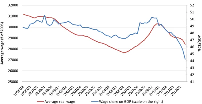
(15) Economies 2014, 2. 161. As Figure 8 shows, during 2000–2007 the participation of workers in the distribution of national income (Compensation of employees/GDP) and the average real wage both recorded almost continuous declines. This is an interesting fact in a period of economic prosperity, but it is along the lines of what happened in the U.S. and has been thoroughly analyzed in the literature. Besides, this downward trend intensified after the first years of the last crisis. Figure 8. Average real wage and wage share in the Spanish gross domestic product (GDP). 52. 32000. 51 50 49. 30000. 48 29000. 47. 28000. 46. %CE/GDP. Average wage (€ of 2005). 31000. 45 27000. 44 43. 26000. 42 41. 25000. Average real wage. Wage share on GDP (scale on the right). Source: own ellaboration with data from INE and OCDE (deflator: CPI).. According to the data, there is certainly an initial phase of the crisis in which average mean salaries and the wage share clearly increase. The increase in real wages can be explained from a statistical methodology problem. On the other hand, the increase in the GDP wage share is due to the strong fall in corporate profits caused by the crisis itself. However, after this first adjustment period, the downward trend in both cases is unequivocal.7 We can see that ultimately, crises have strong effects on workers: first, the number of employees is affected and, later, the salaries of those who have kept their jobs decline. In the light of the evolution of these indicators, it seems undeniable that the really high growth rates of consumption, demand and ultimately of output that Spain experienced between 2000 and 2008 could hardly have existed if it were not for the easy access to credit by families, which offered them a way of supplementing their incomes. 7. Since the average wage is a statistical mean, it is relevant to know how the variable is distributed. If all wage earners had the same wages, an increase or decrease in employment would have no effect on average wages. However, if the distribution of wages is really dispersed, final effects are very different. In Spain the labor market has a dual structure. On the one hand, we have permanent workers (with higher wages) and temporary workers (with lower wages). At the beginning of a crisis, the first who suffer the effects are temporary workers: they lose their jobs and average wages statistically rise. However, as the crisis goes on, the increase in unemployment lowers nearly all salaries, so average wages decrease again..

(16) Economies 2014, 2. 162. Therefore, if we combine these data with the family indebtedness by income segments, the evidence obtained for the Spanish case suggests that the growth of consumption in a period of stagnation in real wages was based on the expansion of credit and in the indebtedness of most of the families with lower income levels. 4. Income and Consumption Inequality Since liquidity constraints have been considerably relaxed for an important part of the Spanish households during 2000–2008, and since households have reacted to this situation by increasing their indebtedness (either to level out their consumption throughout their lives or because of any other factor), it should follow that consumption inequalities have grown less or decreased more than income inequalities. If data confirm this, we could be talking about the existence of favorable empirical evidence for a leveling effect of credit. As a starting point for the analysis of income inequalities in Spain, we use the Gini index data provided by Eurostat (Figure 9). Between 2003 and 2007 (expansion stage), variations are insignificant. On the contrary, from 2008 onwards inequalities grow sharply, a fact which is consistent with the effects that unemployment has on this variable. Figure 9. Gini index for the Spanish economy. 35 34 33 32 31 30 29 2003. 2004. 2005. 2006. 2007. 2008. 2009. 2010. 2011. Spain. Source: Eurostat.. From this finding, a possible reading of the fact that inequalities did not decrease during the expansion period is that the new jobs that were created offered low wages. This is consistent with the idea that the recipients of these wages financed increasing levels of consumption with recourse to borrowing. For the purposes of comparing the evolution of income and consumption inequalities, the information given by the Gini index can be completed with micro-data from the EFF, since this source provides detailed data of both variables (income and consumption) that can be grouped into percentiles of income. Firstly, we have estimated the values of the S80/S20 indicator in terms of income. This indicator is used according to the Eurostat definition: the ratio of total income received by 20% of the population.

(17) Economies 2014, 2. 163. with the highest income (top quintile) with respect to the total income received by 20% of the population with the lowest income (bottom quintile). Income is understood as adjusted gross income (since the EFF does not provide data about taxes, we cannot calculate disposable income in this case). This income is what Banco de España understands as “household total income”, that is, the sum of work-related income and non-work-related income. When making inequality calculations, it is more appropriate to consider the equivalent gross income, that is, the result of dividing the total household income by the number of its members (weighting as 1 the head of the family, 0.5 the rest of individuals above the age of 14 years and 0.3 the individuals under 14 years living at home). This is the OECD criterion, which is also followed by Eurostat. These weightings exist in order to recognize the economies of scale derived from family life. This way, household income is converted into a “standard income” of “same-size households”. The problem inherent in the comparison of very different households is thus solved. Using the available data from the three waves of the survey, and following the methodology previously described, we have first calculated the income inequality indicator S80/S20 (understanding income as equivalised gross income). Secondly, we have calculated a S80/S20 indicator for consumption. This indicator is the quotient between the total consumption of the individuals in the highest income quintile and the consumption of the individuals in the lowest income quintile. Logically, for the calculation of consumption, the variable “annual household consumption” has been adjusted in the same way as the annual income. The results can be seen in Figure 10. The first relevant aspect is that consumption inequality is lower than income inequality. The most basic economic theory points out that marginal propensity to consumption becomes lower as income becomes higher and, therefore, lower income individuals will consume a greater proportion of their income than higher income individuals. On the other hand, the role played by public redistribution in this difference should not be overlooked.8 With respect to the evolution of these indicators, it is clearly visible that consumption inequalities remained almost stable during the period, especially when compared with income inequalities, which increased significantly between 2002 and 2005 and later decreased in 2008’s wave.9 However, the indicator S80/S20 could suffer from a problem of lack of generality when measuring the evolution of inequality, given that only the income received by the top and bottom income quintiles, which exhibit particular behaviours derived from their extreme position in the distribution of income, is taken into account for its calculation. For this reason, in order to take into account the totality of the income groups, we also calculated the ratio between the total income of individuals over the median and individuals below the median (S50/S50, adapting Eurostat’s terminology to the matter that occupies us). The values of the S50/S50 ratio, which are logically smaller in value than S80/S20, point in the same direction as the latter and allow us, in general, to extrapolate the aforementioned results.. 8 9. Brzozowski, M. et al. [43] offer evidence for this for the Canadian case. It should be noted that the indicators do not exactly match in time. Income data refer to the year before the survey, while consumption data are associated with the same year in which the survey takes place (specifically, in part to the 12 months before each household answers the questionnaire and in part to multiplying by 12 the average monthly consumption in the moment the survey takes place)..

(18) Economies 2014, 2. 164. Figure 10. S80/S20 and S50/S50 income and consumption indicators. 10 9 8 7 6 5 4 3 2 1 0 2002. 2005. 2008. Income S50/S50. Consumption S50/S50. Income S80/S20. Consumption S80/S20. Source: own ellaboration from EFF micro-data.. 5. Household Debt and Consumption Inequality: Some Empirical Evidence In order to conduct a multivariate analysis with the aim of possibly making any causality statement on the influence of household debt on consumption, we estimate a reduced form expression for household consumption. The choice of explanatory variables is based in a wide literature that suggests that a household’s consumption in any period depends on a number of factors. 10 Particularly, we assume that household consumption depends on current income, wealth, expectations of future income and the ability to smooth consumption in the face of income shocks. Specifically, Consum = β0 + β1Labinc + β2Capinc + β3Finwealth + β4Reawealth + β5Incexpect + β5 Debt + X + ε (1) where, Consum is household consumption defined as the sum of durable and non-durable consumption over the 12 months prior to the survey. Labinc is the sum of labour income of the household (including proper wages, but also fringe benefits, unemployment benefits or income obtained by unemployed people in other ways). Capinc is defined as all other sources of income for the household that are not derived from labor (interest, dividends, etc.). It was computed as the difference of total household income and labor income as previously defined. Finwealth is the household financial wealth (bank accounts, stocks, bonds, etc.). Realwealth is the household real wealth (housing, equipment, vehicles, etc.). Incexpect is a dummy variable that takes value 1 if the members of the household are expecting to have a higher income in the future and 0 otherwise. Debt is the sum of the household liabilities (either as a home mortgage or for other reasons). X is a vector of socio-demographic variables. All variables are defined in equivalised terms, following the OECD-modified scale that is used by Eurostat (the first adult is weighted as 1, all other individuals aged 14 or more are weighted as 0.5 and 10. See Browning and Lusardi [44] for an overview about micro-determinants of consumption..

(19) Economies 2014, 2. 165. children are weighted 0). For ease of computation, we consider a person to be 14 if he was 14 at the beginning of the year of the survey. We estimate Equation (1) using an ordinary least squares (OLS) procedure and the results are summarized in Table 3. For each year we estimate two models: a baseline specification (Model I) in which we include debt such as it was above defined and a modified version of it in which we consider family indebtedness by income segments (Model II). According to results reported in Table 3, we observe that all the variables proxying household current income and wealth are significant and have the expected sign. Particularly, it is interesting noting that the labor income—mainly wages—influence on households consumption decreases in 2005. Furthermore, in the early 2000s, household debt has a significant and negative effect on consumption. This effect becomes positive from 2005 and its influence seems to increase over time. To some extent, these results for the baseline model are consistent with the hypothesis of a substitution of income for debt in the Spanish economy during the last expansionary phase of the economic cycle. Table 3. Estimates of the influence of debt on household consumption. Dependent Variable: Households consumption (Consum) 2002. 2005. 2008. Regressor. Model I. Model II. Model I. Model II. Model I. Model II. Labincome. 0.19611*** (0.0192). 0.20035*** (0.019). 0.13117*** (0.009). 0.13358*** (0.009). 0.15198*** (0.0068). 0.15044*** (0.0068). −0.0006 (0.009). 0.00119 (0.009). 0.03759*** (0.0041). Capincome. 0.01833*** (0.005). 0.01971*** (0.006). 0.03828*** (0.004). Finwealth. 0.02506*** (0.0005) 0.02499*** (0.0005) 0.00684*** (0.0004). 0.0069*** (0.0004). 0.0011*** (0.00039) 0.00114*** (0.00039). Realwealth. 0.01197*** (0.001). 0.01211*** (0.001) 0.00564*** (0.0005) 0.00562*** (0.0005) 0.00029*** (0.00006) 0.00029*** (0.00006). Incexpect. −803.31* (444.19). −786.71* (443.97). 483.08 (303.59). 488.12 (304.36). −50.667 (284.82). −19.22 (285.11). Debt. −0.0313*** (0.005). −0.0347*** (0.006). 0.00537** (0.003). 0.00318 (0.0028). 0.01473*** (0.0009). 0.01502*** (0.0009). Debt q2. 0.0607** (0.026). 0.0164* (0.0088). −0.00339 (0.007). Debt q3. 0.04701 (0.036). 0.0188 (0.0125). −0.0114 (0.0084). Debtq4. 0.04693 (0.038). 0.0049 (0.018). −0.01944* (0.012). Debtq5. 0.04208 (0.066). 0.0130 (0.017). −0.02604 (0.019). Age. −4.701*** (18.8). −1.2293*** (19.045). −78.313 (12.445). −69.91 (12.57). 66.05*** (11.06). 62.53*** (11.21). Education. −58.18 (65.87). −49.903 (66.014). 192.38*** (44.59). 195.52*** (44.72). 401.05*** (37.46). 394.27*** (37.56). Salaried. −572.22 (556.72). −563.7 (556.72). −872.12** (358.63). −886.20** (358.62). 542.88* (322.64). 557.73* (322.71). Selfemployed. −1388.7* (742.76). −1397.24* (742.36) 1434.07*** (485.74). 1475.6*** (486.16). 3185.33*** (451.32). 3176.99*** (451.52). Unemployed. −1546.83* (900.91). −1506.54* (903.21) −1019.36* (618.02). −1027.77* (618.2). −132.72 (465.87). −107.74 (466.41). 8664.37*** (1248.16) 7929.52*** (1278) 5333.84*** (793.95). 5015.9*** (811.4). 314.35 (732.96). 649.05 (750.69). Constant Number of observations F 2. R. 2743. 2743. 3323. 3323. 3252. 3252. 464.13 (0.0000). 341.40 (0.0000). 187.52 (0.0000). 137.93 (0.0000). 217.4 (0.0000). 159.92 (0.0000). 0.6515. 0.6525. 0.3839. 0.3849. 0.4247. 0.4257. *** Significant at 1 % level; ** significant at 5 % level; * significant at 10 % level.. It is worth noting the sharp fall in the value of R2 in regressions based on 2005 and 2008 samples. It is quite possible that there may be other important factors that influence household consumption besides those captured in the baseline model. Therefore, to draw substantive conclusions about the.

(20) Economies 2014, 2. 166. effect on consumption of changes in household debt, the model specification should be augmented with additional control variables. In order to obtain some additional evidence of the potential effect on households’ consumption of households’ indebtedness, we consider an alternative to the baseline specification. With this purpose, in Model II we include five interaction terms: debtq1, debtq2, debtq3, debtq4 and debtq5 that are the result of multiplying debt by a dummy variable that expresses the household income quintile. Indeed, regression in model II examines whether the effect of changing household debt on consumption varies across income quintiles. In other words, by including interactions between debt and income quintiles, we can check whether the regression functions relating debt and household consumption are different for low and high household income levels. As can be seen in Table 3, the difference between the estimated effects across income segments is not statistically significant. As we have discussed in Section 3, in the Spanish case, indebtedness (in terms of household income) is mostly concentrated in the lower income quintiles. If we combine these data with the results derived from our econometric estimates, we obtain some evidence suggesting that the growth of consumption in Spain over a period of stagnation in real wages was partially based on the expansion of credit and on the indebtedness of most of the families with lower income levels. 6. Conclusions The process of growing indebtedness which was experienced by Spanish households in the last expansion phase of the economy and its subsequent correction with the onset of the crisis has had important implications in several fields. This article has mainly focused on the search for clues in a two-way direction: on the one hand, regarding the role played by inequalities in the process of household indebtedness and, on the other hand, regarding the possible distributive consequences of financial conditions. More specifically, the analysis that has been developed throughout this work allows us to obtain some empirical evidence that, without being completely conclusive, gives some credibility to the hypothesis that consumption inequalities did not respond to variations in income inequalities, but were kept “artificially” low during the period under study. This evidence would be compatible with the existence of a levelling effect of credit during that period, in the sense used by Brown [20] or predicted by the model in Rancière and Kumhof [24]. Our empirical analysis provides some preliminary evidence of the phenomenon of substitution of debt for wages as a determinant of households’ consumption in the Spanish economy during the last expansionary phase of the economic cycle. Moreover, the observed differences in the evolution of income and consumption over that period of time can be explained under the hypothesis that within a context of growing income inequality consumption inequality only can be reduced by a general surge in consumption-related borrowing by low and middle-income households. Furthermore, the favorable financial conditions that prevailed during that stage helped to reduce the liquidity constraints that affect mostly lower-income households. This would be a factor that may have contributed to containing the growth of inequalities measured in terms of consumption. Finally, it should be noted that, if the main hypothesis of this article is true, the end of easy financial conditions since the beginning of the current crisis would make inequalities worse. On the one hand, it.

(21) Economies 2014, 2. 167. would worsen income inequalities because of the already proven effect of unemployment over them, widely covered in literature. On the other hand, it would worsen consumption inequalities because of the main argument developed in this article. From the point of view of supply, financial conditions are more restrictive nowadays and, from the point of view of demand, many of the factors that drove individuals to finance their consumption with credit have been moderated (for example, it is likely that wealth effect will have changed its sign because of the reduction in the price of real estate assets). As a result of these factors, families resort less to borrowing in order to finance consumption. Therefore, depending on the extent to which households, especially those of lower income and wealth, are suffering “liquidity constraints” again, they will not be able to distribute their consumption as they would like to. This way, these households would be limited to the use of their current income which, in many cases, has suffered a negative impact. In these circumstances, the future increase in consumption inequalities will be more than likely. The three available EFF have been conducted between 2002 and 2008, which is too short a time to make any meaningful predictions. In this sense, although the publication of the EFF 2011 will allow a more exhaustive study to be carried out of the changes arising from the new economic situation that Spain faces, it is likely that high household indebtedness will be one of the factors that has aggravated the severity of the effects of the increase of unemployment and the sharp correction in prices of real estate assets on inequalities. In any case, our findings should be recognized as tentative because we do not yet have any evidence in terms of causality, and the empirical evidence shown could be compatible with other interpretations. Acknowledgments The authors are grateful to the journal editor and three anonymous reviewers for their helpful comments. All remaining errors are our own. Author Contributions Both authors (G.P.P. and J.M.S.) contributed equally to the work presented in this paper. Particularly, G.P.P. and J.M.S. made substantial contributions to conception and design, acquisition of data and analysis and interpretation of data. Both, G.P.P. and J.M.S. discussed the results and implications and commented on the manuscript at all stages. Finally, G.P.P. and J.M.S. drafted the article and revised it critically for important intellectual content. The order of authors was established following an alphabetical criterion. Conflicts of Interest The authors declare no conflict of interest. References 1.. King, R.G.; Levine, R. Finance and growth: Schumpeter might be right. Quart. J. Econ. 1993, 108, 717–737..

(22) Economies 2014, 2 2. 3. 4. 5. 6. 7.. 8. 9. 10. 11.. 12.. 13.. 14.. 15. 16. 17. 18.. 19.. 168. Heathcote, J.; Perri, F.; Violante, G.L. Unequal we stand: An empirical analysis of economic inequality in the United States, 1967–2006. Rev. Econ. Dyn. 2010, 13, 15–51. Agnello, L.; Sousa, R.M. How do banking crises impact on income inequality? Appl. Econ. Lett. 2012, 19, 1425–1429. Barba, A.; Pivetti, M. Rising household debt: Its causes and macroeconomic implications— A long-period analysis. Camb. J. Econ. 2009, 33, 113–137. Rajan, R.G. Fault Lines—How Hidden Fractures Still Threaten the Global Economy; Princeton University Press: Princeton, NJ, USA, 2010. Galbraith, J.K. Inequality and Instability: A Study of the World Economy just before the Great Crisis; Oxford University Press: New York, NY, USA, 2012. Debelle, G. BIS Working Papers. No 153. Macroeconomic Implications of Rising Household Debt. Available online: http://www.ecri.eu/new/system/files/46+2004_Macroecon_impl_rising_ household_debt.pdf (accessed on 15 June 2013). Survey of Household Finances. Available online: http://www.bde.es/bde/en/areas/estadis/ Otras_estadistic/Encuesta_Financi/ (accessed on 15 June 2013). Pijoan-Mas, J.; Sánchez-Marcos, V. Spain is different: Falling trends of inequality. Rev. Econ. Dyn. 2010, 13, 154–178. Farré, L.; Vella, F. Macroeconomic conditions and the distribution of income in Spain. Labour 2008, 22, 383–410. Bonhomme, S.; Hospido, L. The Cycle of Earnings Inequality: Evidence from Spanish Social Security Data. Available online: http://www.bde.es/f/webbde/SES/Secciones/Publicaciones/ PublicacionesSeriadas/DocumentosTrabajo/12/Fich/dt1225e.pdf (accessed on 10 July 2013). Ayala, L.; Cantó, O.; Rodríguez, J.G. Poverty and the Business Cycle: The Role of the Intra-Household Distribution of Unemployment. ECINEQ WP 2011-222. Available online: http://www.ecineq.org/milano/WP/ECINEQ2011-222.pdf (accessed on 13 August 2013). Addabo, T.; García-Fernández, R.; Llorca-Rodríguez, C.; Maccagnan, A. The Impact of the Crisis on Unemployment and Household Income in Italy and Spain. ECINEQ WP 2011-235. Available online: http://www.ecineq.org/milano/WP/ECINEQ2011-235.pdf (accessed on 13 August 2013). Fundación Alternativas 1er Informe sobre la Desigualdad en España. Available online: http://www.falternativas.org/la-fundacion/documentos/libros-e-informes/1er-informe-sobre-ladesigualdad-en-espana-2013 (accessed on 23 September 2013). Friedman, M. A Theory of the Consumption Function; Princeton University Press, Princeton, NJ, USA, 1957. Ando, A.; Modigliani, F. The life-cycle hypothesis of saving: Aggregate implications and tests. Am. Econ. Rev. 1963, 103, 55–84. Modigiliani, F. The life cycle hypothesis of saving, the demand for wealth and the supply of capital. Soc. Res. 1966, 33, 160–217. Foster, J.B.; Magdoff, H. Working Class Households and the Burden of Debt. Available online: http://monthlyreview.org/2000/05/01/working-class-households-and-the-burden-of-debt/ (accessed on 28 October 2013). Foster, J.B. The Household Debt Bubble. Available online: http://monthlyreview.org/ 2006/05/01/the-household-debt-bubble/ (accessed on 29 October 2013)..

(23) Economies 2014, 2. 169. 20. Brown, C. Does income distribution matter for effective demand? Evidence from the United States. Rev. Polit. Econ. 2004, 16, 291–307. 21. Iacoviello, M. Household debt and income inequality, 1963–2003. J. Money Credit Bank. 2008, 40, 929–965. 22. Barba, A.; Pivetti, M. Changes in income distribution, financial disorder and crisis. In The Global Economic Crisis: New Perspectives on the Critique of Economic Theory and Policy; Brancaccio, E., Fontana, G., Eds.; Routledge: Londres, Argentina, 2011; pp. 81–97. 23. Barba, A.; Pivetti, M. Distribution and accumulation in post-1980 advanced capitalism. Rev. Keynes. Econ. 2012, 1, 126–142. 24. Kumhof, M.; Rancière, R. Inequality, Leverage and Crises. IMF Working Paper WP/10/268. Available online: https://www.imf.org/external/pubs/ft/wp/2010/wp10268.pdf (accessed on 3 September 2013). 25. Shapiro, M.D. The permanent income hypothesis and the real interest rate: Some evidence from panel data. Econ. Lett. 1984, 14, 93–100. 26. Campbell, J.Y.; Mankiw, N.G. Consumption, Income and Interest Rates: Reinterpreting the Time Series Evidence. MIT Press. Available online: http://www.nber.org/chapters/c10965.pdf (accessed on 4 November 2013). 27. Bacchetta, P.; Gerlach, S. Consumption and credit constraints: International evidence. J. Monet. Econ. 1997, 40, 207–238. 28. Boone, L.; Girouard, N.; Wanner, I. Financial Market Liberalisation, Wealth and Consumption. OECD Economics Department Working Papers, No. 308, OECD Publishing, 2001. Available online: http://www.oecd-ilibrary.org/docserver/download/5lgsjhvj80g8.pdf?expires= 1405484028&id=id&accname=guest&checksum=51B309767F3E30717E1A3C5FAA8FA1F5 (accessed on 12 September 2013). 29. Brady, R.R. Structural breaks and consumer credit: Is consumption smoothing finally a reality? J. Macroecon. 2008, 30, 1246–1268. 30. Brady, R.R. Consumer credit, liquidity and the transmission mechanism of monetary policy. Econ. Inq. 2010, 49, 246–263. 31. Aron, J.; Duca, J.V.; Muellbauer, J.; Murata, K.; Murphy, A. Credit, housing collateral and consumption: Evidence from Japan, the UK and the US. Rev. Income Wealth 2011, 58, 397–423. 32. Brown, C. Financial engineering, consumer credit, and the stability of effective demand. J. Post Keynes. Econ. 2007, 29, 429–455. 33. Galbraith, J.K. With Economic Inequality for All. Available online: http://www.njfac.org/galineq.htm (accessed on 30 September 2013). 34. Coibion, O.; Gorodnichenko, Y.; Kueng, L.; Silvia, J. Innocent Bystanders? Monetary Policy and Inequality in the US. Available online: http://www.nber.org/papers/w18170 (accessed on 2 May 2013). 35. Pichette, L. Are Wealth Effects Important for Canada? Available online: http://www.bankofcanada.ca/ wp-content/uploads/2010/06/pichettee.pdf (accessed on 23 June 2013). 36. Carroll, C.D.; Otsuka, M.; Slacalek, J. How large are housing and financial wealth effects? A new approach. J. Money Credit Bank. 2011, 43, 55–79..

(24) Economies 2014, 2. 170. 37. Case, K.E.; Quigley, J.M.; Shiller, R.J. Comparing wealth effects: The stock market versus the housing market. Adv. Macroecon. 2005, 5, 1–34. 38. Bernanke, B.; Gertler, M. Agency costs, net worth, and business fluctuations. Am. Econ. Rev. 1989, 79, 14–31. 39. Antzoulatos, A.A. Consumer credit and consumption forecasts. Int. J. Forecast. 1996, 12, 439–453. 40. Ludvigson, S. Consumption and credit: A model of time-varying liquidity constraints. Rev. Econ. Stat. 1999, 81, 434–447. 41. Banco De España. Boletín Económico. Encuesta Financiera de las Familias (EFF) 2005: Métodos, Resultados y Cambios entre 2002 y 2005. Available online: http://www.bde.es/f/webbde/ SES/estadis/eff/Separata_EFF_2007.pdf (accessed on 23 October 2013). 42. Banco de España. Boletín Económico. Encuesta Financiera de las Familias (EFF) 2008: Métodos, Resultados y Cambios desde 2005. Available online: http://www.bde.es/f/webbde/SES/ estadis/eff/eff2008_be1210.pdf (accessed on 23 October 2013). 43. Brzozowski, M.; Gervais, M; Klein, P.; Suzuki, M. Consumption, income and wealth inequality in Canada. Rev. Econ. Dyn. 2010, 13, 52–75. 44. Browning, M.; Lusardi, A. Household saving: Micro theories and micro facts. J. Econ. Lit. 1996, 34, 1797–1855. © 2014 by the authors; licensee MDPI, Basel, Switzerland. This article is an open access article distributed under the terms and conditions of the Creative Commons Attribution license (http://creativecommons.org/licenses/by/3.0/)..

(25)