Finite element formulation for large displacement analysis

(1)

—————————————————–

Finite Element Formulation

for Large Displacement Analysis

—————————————————–

Mario Gomez Botero

Department of Mechanical Engineering

EAFIT University

(2)

(3)

In structural engineering, shells are usually curved objects which can sup-port remarkable external forces without fracture or damage. Due to this re-markable stiffness behaviour and the low amount of material used in the fab-rication process, nowadays shell structures are getting lots of followers in the engineering world. In consequence, scientists and the industry in general are keen with the idea of developing efficient and accurate models to predict their behaviour.

In the manufacturing industry, inspection procedures are becoming more common every day. This task constists on measuring how much difference ex-ists between the original-ideal object specified by the designer, and the object that just comes out from the manufacturing process. Generally, this goal is achived by placing the manufactured part in the location where it was de-signed to be, such as the assamblage of a machine. Subsequently, a 3–D scan of the placed part is made. The registered measurments are compared with the CAD geometry of the original-ideal object in order to acept or reject the manufactured part. However, this procedure represents an inefficient and very time consumig process. If instead, the part is scanned when it just comes out from the fabrication process, and the scanned geometry is placed into the assemblage via a Finite Element software; a more efficient procedure could be achieved assuming that the simulation is fast and reliable. The goal of this work is to provide this virtual inspection enviroment.

Given the nature of the manufactured parts, the physics of the problem cor-responds to shell structures subjected to large displacements. In consequence, the formulation, implementation, and validation of a shell element based on a large displacement hypothesis have to be fully understood. Nevertheless, before arriving to shell elements, it has been considered as convenient to com-prehend the Finite Element formulation proposed in the literature for bars, beams, and plane stress elements.

(7)

Contents 7

to reach the same results they publish without giving many clues about the right way to get to that point. This text gets into the detail of the mathemat-ics required to deal with finite deformations and large displacements applied to the Finite Element Method; for that purpose, it was necessary to under-stand several author’s point of view and sometimes comprehend very different mathematical notations to explain the same idea. The final products obtained (both the written report and the C++ shell program) represent a big shortcut for those who want to gain good knowledge and understanding of the Finite Element Method under the large displacement hypothesis.

(8)

(9)

Chapter 1 Introduction to the Variational

Formulation

The study of mechanics has always been a branch of interest for scientists. In general, the problems found therein can be expressed through mathematical models which can be written in terms of partial differential equations (PDE). Two main lines of study have been developed to generate these equations: The first one, and the most recognised, is the one based on Newton’s laws of motion, which seeks for all the forces acting on every particle within a domain. The differential formulation has its foundations in this trend.“The second branch of mechanics, usually called analytical mechanics, which bases the entire study of equilibrium and motion on two fundamental scalar quantities, the kinetic energy and the potential energy”(Lan86), represents the basis of the variational formulation.

1.1 Minimum Total Potential Energy

Princi-ple

The Calculus of Variations has come up as an efficient tool that can be applied to a large amount of mathematical problems. Fortunately for engineers, in gen-eral it is possible to express the basic principles of mechanics as a mathematical variational problem. In such a way, this physical phenomenom acquires a big mathematical meaning which allows to understand more clearly how nature works. The principle of Minimum Total Potential Energy (MTPE) is a fun-damental concept used in structural mechanics. It states that an object will deform into a position where the total potential energy is minimised. In

(10)

10 Chapter 1. Introduction to the Variational Formulation

sical mechanics, this principle can be expressed in terms of the displacement field ~u = ui, and at most, in terms of its first derivative with respect to the

spatial coordinates, that is ∂ui

∂xj. This aspect will be seen more clearly when

defining the energies considered by the MTPE principle.

Mathematically, this principle asserts that the Total Potential Energy Π of the system being analysed, equals to the difference between the strain energy

U stored in the deformed object, and the potential energy of the loads W. That is,

Π(ui,∂ui/∂xj)=U(ui,∂ui/∂xj)−W(ui,∂ui/∂xj). (1.1)

According to what it is expressed above, the functional Π(ui,∂ui/∂xj) may be

understood as a master function whose domain is constituted by the vector functions ui and ∂ui/∂xj. It is also important to remark that Π remains

unchanged during motion of the object; therefore δΠ = 0. For that reason, when a loss of potential energy occurs, that quantity of energy is gained by the strain energy and vice versa.

Even though the equations for mechanical problems can be generated via a differential formulation, a better way to face the problem and get to the truly core of the concepts involved therein would be the Calculus of Variations. Indeed, for engineering purposes, the MTPE principle can be specialised into the the principle of virtual displacements using the Calculus of Variations. This principle is widely employed in continuum mechanics, mainly because it serves as a basis to state the equilibrium equations in a deformable medium.

In order to see how the the principle of virtual displacements works, it is possible to think of a particle which is located at point P1 at a time t1, and

has a velocity v1. The particle will move to point P2 at a time t2. An infinity

(11)

1.2. Derivation of the Principle of Virtual Displacements 11

1.2 Derivation of the Principle of Virtual

Dis-placements

The variational problem to be solved in structural mechanics consists on finding a functionui for which the functional Π(ui,∂ui/∂xj)is a maximum, is a minimum,

or has a saddle point. The condition to get to the governing equations is

δΠ(ui,∂ui/∂xj) = 0,

and due to the calculus of variations

δΠ₍

ui,∂ui/∂xj) =

∂Π

∂ui

δui+

∂Π

∂(∂ui/∂x)

δ(∂ui/∂x)

“It must be noted that δui stands for variations on ui that are arbitrary except

that they must be zero at and corresponding to the state variable boundary con-ditions. The second derivatives of Πwith respect to ui then decide whether the

solution corresponds to a maximum, a minimum, or a saddle point.”(Bat96). In general, the total potential energy of a 3–D structural body, can be expressed as

Π(ui,∂ui/∂xj)

| {z }

total potential energy

=

Z

V

1

2τijeijdV

| {z }

strain energy

−

Z

V

f_iBuidV +

Z

S

fSf

i u Sf

i dS

| {z }

total potential of the loads

=

Z

V

1

2CijmnemneijdV −

Z

V

f_iBuidV −

Z

Sf

fSf

i u Sf

i dS,

wherefB

i represents the body forces per unit volume,f Sf

i are the surface forces

per unit area, and eij = 1₂(_∂x∂ui_j + ∂uj

∂xi) =

1

2(ui,j +uj,i). As it was stated before,

note that the energies considered by MTPE principle can be written at most in terms of ∂ui

∂xj. The first variation of Π with respect to the displacement field

is

δΠ(ui,∂ui/∂xj) = 0 =

Z

V

1

2Cijmnemnδ(eij)dV +

Z

V

1

2Cijmnδ(emn)eijdV

−

Z

V

f_iBδuidV −

Z

Sf

fSf

i δu Sf

i dS.

(12)

first variation of Π can be rewritten as

0 =

Z

V

1

2τijδ(eij)dV +

Z

V

1

2Cmnijeijδ(emn)dV −

Z

V

f_iBδuidV −

Z

Sf

fSf

i δu Sf

i dS

=

Z

V

1

2τijδ(eij)dV +

Z

V

1

2τmnδ(emn)dV −

Z

V

f_iBδuidV −

Z

Sf

fSf

i δu Sf

i dS,

and taking into account that ij and mn are free indices, the final expression for the first variation of Π is obtained,

Z

V

τijδ(eij)dV

| {z }

internal virtual work

=

Z

V

f_iBδuidV +

Z

Sf

fSf

i δu Sf

i dS.

| {z }

external virtual work

(1.2)

The above expression is known as the principle of virtual displacements, and constitutes a general expression for the development of equations used by the Finite Element Method applied to structural mechanics.

1.3 Derivation of the equilibrium equations from

the principle of virtual displacements

Considering the symmetry of the Cauchy stress tensor (τij =τji), it is possible

to say that

τijδeij =τijδ

1

2(ui,j+uj,i)

=τij

1

2[(δui,j+δuj,i)]

= 1

2τijδui,j+ 1

2τijδuj,i = 1

2τijδui,j

| {z }

term 1

+1

2τjiδuj,i

| {z }

term 2 ,

but taking a closer look, it can be seen that term 1 and term 2 are independent. It means that the indices i and j in term 1 are not related to indices i and j

in term 2. Hence, they are similar terms, thus

τijδeij =τijδui,j.

Therefore, Equation 1.2 can be expressed as

Z

V

τijδui,jdV =

Z

V

f_iBδuidV +

Z

Sf

fSf

i δu Sf

(13)

1.3. Derivation of the equilibrium equations from the principle of

virtual displacements 13

now if the mathematical identityτijδui,j = (τijδui),j−τij,jδui is used, it yields

to

Z

V

[(τijδui),j−τij,jδui] dV =

Z

V

f_iBδuidV +

Z

Sf

fSf

i δu Sf

i dS,

and by the divergence theorem

Z

S

(τijδui)njdS−

Z

V

τij,jδuidV =

Z

V

f_iBδuidV +

Z

Sf

fSf

i δu Sf

i dS

where Sf ∪Su =S, and Sf ∩Su = 0. Sf corresponds to the surface where the

loads are applied, andSu is the surface where the displacements are prescribed,

hence

Z

Sf

(τijnj −f Sf

i )δu Sf

i dS+

Z

Su

τijnjδuSiudS =

Z

V

(τij,j +fiB)δuidV. (1.3)

Looking for a good interpretation of Equation 1.3, it is essential to remember the fundamental theorem of the calculus of variations:

Theorem 1 If f(x) is continuous in [a, b] and if

Z b

a

f(x)α(x)dx= 0

for every continuous function α(x) in [a, b] that vanishes in a and b, hence f(x)= 0 for every x∈[a, b].

This theorem can be naturally extended to several variables (TG07). To ob-tain the differential equation which governs this 3–D structural problem, it is indispensable to check out under what particular conditions Equation 1.3 vanishes for any possible perturbation δui. Choosing perturbations δui that

ara zero atSu and Sf, the left hand side of 1.3 vanishes. That isδuSiu = 0 and

δuSf

i = 0. Now, it is time to search under what conditions

R

V(τij,j+f B

i )δuidV

vanishes for any δui that satisfies δuSiu = 0 and δu Sf

i = 0. The fundamental

theorem of the calculus of variations guarantees that

τij,j+fiB = 0. (1.4)

(14)

everywhere except at Sf, and according to the fundamental theorem of the

calculus of variations; it is possible to state that the problem is accomplished with the natural boundary condition

τijnj −f Sf

i = 0,

and the prescribed essential boundary conditions.

When utilising a variational approach, two different kinds of Boundary Conditions can generated: The essential and the natural boundary conditions. Consider that in the functional Π, the highest derivative of the state variable with respect to a space variable is of order m. That problem is known as a Cm−1 _{variational problem. The essential boundary conditions correspond}

to the prescribed displacements and rotations, for that reason are also called geometric boundary conditions. The order of the derivatives in the essential boundary conditions is, in aCm−1 _{problem, at most}_m₋_{1. On the other hand,}

the natural boundary conditions correspond to the prescribed boundary forces and moments. The highest derivatives are of order m to 2m−1 (Bat96).

Finally, going back to Equation 1.2, is possible to affirm that to be able to find a displacement function ui which is a solution of the problem, “the

internal virtual work must be equal to the external virtual work for arbitrary test or virtual displacement functions δui that are continuous and satisfy the

condition δuSu

i = 0 and δu Sf

(15)

Chapter 2 Displacement Based FEM

In general, when solving an engineering problem, it is necessary to identify and sometimes to develop a mathematical model whose results are close enough to reality. Normally, the mathematical model leads to a set of the mathemati-cal equations that must be solved considering some solution method. In the particular case of structural mechanichs, when using a variational formulation to describe a deformation process, the final system of continuous differential equations generated (see Equation 1.4) establish mathematically the equilib-rium requirements, compatibility conditions, and constitutive relations for all the differential elements within the domain of the object to be deformed.

The Finite Element Method (FEM) emerges as the most popular model used by engineers to solve a system of differential equations. However, to be able to get into the world of the Finite Elements, it is necessary to discretise the system of continuous equations. Of course the final result will not coincide with the exact solution of the model; instead, a very good approximation might be achieved.

In order to discretise the system of continuous equations, the domain of the problem has to be divided into a finite number of elements. Then, a system of finite element equilibrium equations which are deduced from the principle of virtual displacements are applied to each element. Finally, the complete system of equations obtained from the whole amount of elements is solved via some numerical method. In general, the elements used to discretise the domain are basic geometries such as pyramids and prisms for the 3–D cases, or triangles and quadrilaterals for 2–D. The state variables of the problem are usually located at the vertices of the elements, but sometimes they are also located inside the element or over its edges. State variables are those that contain enough information about the system being analysed to enable computation

(16)

16 Chapter 2. Displacement Based FEM

of its behaviour under certain boundary conditions, e.g. the displacements, the strains, etc. The spatial points where the state variables are located are called nodes.

2.1 Finite Element Equations

In this section the general procedure to state the finite element equations for a general 3–D problem will be derived. First, it is appropriate to define the problem that is wanted to be solved: Consider an arbitrary 3–D body which is being deformed because the imposition of some boundary conditions, see Figure 2.1. The body is referred to a Cartesian coordinate system. The displacements are prescribed on surface Su and it is also subjected to surface

forces fSf_{. Furthermore, there exists a body force per unit volume} _fB _acting

over the whole domain. The problem is to calculate the displacements ui of

the body and the corresponding strainseij and stresses τij.

z

x

fSf

Su

Sf

y

Figure 2.1: Geometry of a general 3-D body. Figure taken from reference (Bat96).

As already was said, in Finite Element Analysis (FEA), the body which is going to be analysed is approximated into an assemblage of finite elements. Those elements are composed by nodal points, which can be located over its boundary or within its interior. The displacements ui of every element, are

(17)

2.1. Finite Element Equations 17

points. Then, for an elementm it can be stated that

(m)_u

i = n

X

k=1

hkuki, i= 1,2,3.

where (m)_u

i is measured in a conveniently local coordinate system, hk are

the interpolation base functions, and uk_i correspond to the state variables of elementm. Displacements(m)_u

i =(m)ucan be assembled as the multiplication

of a matrix H and a vector ˆu. That is,

(m)

u=(m)Hu,ˆ (2.1)

where (m)H is called as the displacement interpolation matrix, and ˆu is a vector containing the global displacement components at all nodal points of the assemblage. The size of (m)H and ˆu depends on the space where the problem is being simulated (3–D, 2–D, or 1–D), the total amount of nodes n

of the system, and the number of degrees of freedom (dof) per node used. In the particular case when the problem analysed is in 3–D, with only displacements used as state variables, the size of (m)H would be 3×3n, and ˆu would be of size 3n, thus

ˆ

u= [u1₁, u1₂, u1₃, u₁2, u2₂, u2₃, . . . , u₁n−1, un₂−1, un₃−1, un₁, un₂, un₃].

The Cauchy stress tensor τij and the small strain tensoreij can be written

in vector form, e.g. in the 3–D case eij = e = [e11, e22, e33,2e12,2e13,2e23],

where the fact that eij = eji has been considered. Hence, the corresponding

element strains can be calculated by differentiating Equation 2.1 as

(m)_e₌(m)_B_u,_ˆ _(2.2)

where (m)_B _{is the strain-displacement matrix}1_{. The size of} (m)_B _{depends on}

the problem being analysed, for example a 3–D element with only displacement degrees of freedom would have a size of 6×3n.

Virtual displacements and virtual strains are calculated similarly; hence

(m)_δu₌(m)_{H δ}_u_ˆ _(2.3)

(m)_δe₌(m)_{B δ}_u,_ˆ _(2.4)

and the stresses are related to the strains via the material constitutive relation

(m)_τ

ij =(m)Cijmn(m)emn, (2.5)

(18)

18 Chapter 2. Displacement Based FEM

or written in matrix notation

(m)

τ =(m)C(m)e. (2.6)

where (m)C is the material constitutive matrix. In the 3–D case, (m)C is a 6×6 square matrix. Now, if tensors τij and eij are expressed in vector form,

Equation 1.2 (principle of virtual displacements) can be rewritten as

Z

V

τ δedV =

Z

V

fBδudV +

Z

Sf

fSf_δuSf_dS.

Next, substitution of equations 2.1 to 2.6 into the above expression, and con-sidering the whole assemblage of elements, yields to

n-ele

X

m=1

Z

(m)_V

δuˆT (m)BT

| {z }

(m)_δ_e

(m)

C(m)B (m)uˆ

| {z }

(m)_τ

(m) dV =

n-ele

X

m=1

Z

(m)_V

(m)_fB (m)_HT (m)_δ_u_ˆT (m)_dV₊ n-ele

X

m=1

Z

(m)_S

f

(m)_fSf

h

(m)_HSf

iT

δuˆT (m)dS,

and rearranging terms

δuˆTh

n-ele

X

m=1

Z

(m)_V

(m)

BT (m)C(m)B(m)dViuˆ =

δuˆT

hn-ele_X

m=1

Z

(m)_V

(m)

HT (m)fB(m)dV+

n-ele

X

m=1

Z

(m)_S

f

[(m)HSf_]T(m)_fSf(m)_dS

i

.

(2.7)

“To obtain from 2.7 the equations for the unknown nodal point displacements, the principle of virtual displacements is applied n times by imposing virtual displacements in turn for all components ofδu. In the first applicationˆ δuˆ =e1, in the second application δuˆ = e2, and so on, until in the nth application δuˆ =en”(Bat96). In this way, Equation 2.7 can be expressed as

(19)

2.1. Finite Element Equations 19

where

R=

n-ele

X

m=1

Z

(m)_V

(m)_HT (m)_fB(m)_dV ₊ n-ele

X

m=1

Z

(m)_S

f

h

(m)_HSf

iT

(m)_fSf (m)_dS.

K is known as the stiffness matrix of the element, and is given by

K =

n-ele

X

m=1

Z

(m)_V

(m)_BT (m) _C (m)_B (m)_dV. _(2.9)

In case that concentrated loads are going to be considered, they are written directly in vector Rin the posicion corresponding to the discrete displacement variable ˆu where the concentrated load is applied. This kind of loads were not considered in the functional Π(ui,∂ui/∂xj) because in real world, punctual forces

(20)

(21)

Chapter 3 Large Displacement-based

Nonlinear FEA

In the previous chapter, only small displacements were considered. “The fact that the displacements must be small has entered into evaluation of matrix K and load vectorRbecause all integrations have been performed over the original volume of the finite elements, and the strain-displacement matrix(m)_B _{of each} element was assumed to be constant and independent of the element displace-ments”(Bat96). Therefore, the formulation described therein, applies only to a certain kind of problems with many engineering restrictive characteristics. Hence, a more general formulation considering large displacements represents a better approach to the real conditions of some problems. This fact will be discussed in this chapter; first some basic concepts will be explained, followed by the mathematical formulation of the problem which must be solved. Fi-nally, the formulation for the incremental Total Lagrangian equations will be described, which leads to the Finite Element equations.

3.1 Basic Notions

In large deformation analysis, the domain V of the body is changing contin-uously, as well as its boundary conditions and the external loads. Therefore, if the coordinate system chosen remains stationary and the body is moving in this coordinate frame, the stress and strain measures (τij, eij) used in small

displacement analysis, become useless because they vary under rigid body rotations, which is not allowed by the Principle of Frame Indifference1.

Fur-1_{see (Mal69) for an explanation}

(22)

22 Chapter 3. FEA for Large Displacements

thermore, the small strain tensor eij by definition does not take into account

higher order terms which are necessary in a large deformation analysis. Thus, corresponding stress and strain measures which are invariant under rigid body rotations and with no omission of higher order terms must be defined.

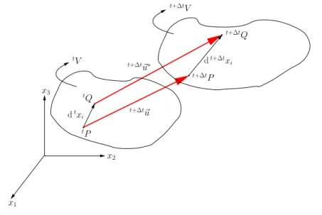
Several different kinds of strain, stress, and some other related quantities have been proposed. This quantities might be defined in terms of the unde-formed configuration (Lagrangian formulation), or in terms of the deunde-formed configuration (Eulerian formulation). The coordinates of the undeformed orig-inal object are known as material coordinates, and therefore are used by the Lagrangian formulation. Instead, Eulerian formulation uses spatial coordinates which are those of the deformed configuration.

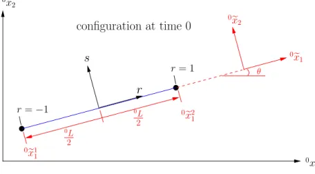
t_x

2 t+∆tx2

t_V

t+∆t_V

t_P_{: (}t_x 1,tx2,tx3)

t_x1 t+∆t_x

1

t+∆t_P_{: (}t+∆_x

1,t+∆tx2,t+∆tx3)

t+∆t_~_u

Figure 3.1: Movement of a point in large displacement analysis.

For this kind of problems it is necessary to employ an incremental formu-lation. A time variable t describes the loading and the motion of the body. The aim is to evaluate the equilibrium positions of the complete body at the discrete time points 0,∆t,2∆t,3∆t, . . . , where ∆t is an increment in time. Towards the solution of the problem, assume that the static and kinematic variables for all time steps from time 0 to timet, inclusive, have been obtained already. Hence, the location of the body for the next equilibrium position corresponding to the discrete time t+ ∆t needs to be reached. This process is applied repetitively until the complete solution path has been solved for (Bat96).

(23)

3.1. Basic Notions 23

quantities are referred to the configuration at time t) in a large deformation analysis can lie very far away from its initial position after deformation t+∆t_u_.

In the classical linear theory of elasticity, the displacements experimented by a deformable body are assumed to be very small. Hence, the final position

t+∆t_P _{of a point in a body lies very close to its initial position} t_P_.

Approx-imations based on the idea of infinitesimal displacement lead to a complete linearisation of the theory of deformation. However, in a more general formu-lation, it is necessary to abandon this restriction (BC99).

Before new stress and strain quantities are defined, some kinematic mea-sures of motion for a body must be outlined:

3.1.1 The Displacement gradient and the Deformation

gradient

The deformation suffered by any particle within a body from timetto timet+ ∆t, is commonly represented by a 3–D vector (see Figure 3.2) with components

t+∆t_u₌t+∆t_u

1ˆı +t+∆tu2ˆ +t+∆tu3ˆk,

where

t+∆t

u1 =t+∆tx1−tx1, t+∆tu2 =t+∆tx2−tx2, t+∆tu3 =t+∆tx3−tx3. (3.1)

Hereafter this point, the amount of deformation t+∆t_u _{will be denoted by} _u_,

or in indicial notation t+∆tui =ui.

In Figure 3.2, it is implicitly assumed that the object with domain t_V _has

already been deformed from its initial state at time 0 to the state at time t. Of course, at time 0 the original domain of the object was 0V. Therefore, the amount of deformation which takes place between time 0 and t is denoted by

t_u ₌t_u

i, and its vectorial components are: t_u

1 =tx1−0x1, tu2 =tx2−0x2, tu3 =tx3−0x3.

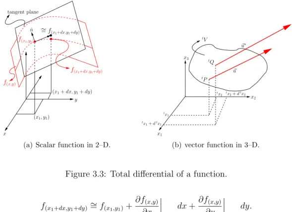
In a Cartesian coordinate system, when analysing the deformation of a body, a particle initially located at a pointt_P _{: (}t_x

1,tx2,tx3) passes to a point

t+∆t_P _{: (}t+∆t_x

1,t+∆tx2,t+∆tx3). Likewise, a particle tQ : (tx1 + dtx1,tx2 + dtx2,tx3+dtx3) passes to a pointt+∆tQ: (t+∆tx1+dt+∆tx1,t+∆tx2+dt+∆tx2,

t+∆t_x

3 +dt+∆tx3), see Figure 3.2. The infinitesimal line tP Q is ordinarily

(24)

t_V

t+∆t_V

dt+∆t_x i t+∆t_P

t+∆t_Q

x2

x1 x3

dt_x i t_P t_Q

t+∆t_~_u∗

t+∆t_~_u

Figure 3.2: Infinitesimal vectors dt_x

i and dt+∆txi.

vector tP Q is denoted by dtxi, and t+∆tP Q is denoted by dt+∆txi. After

deformation, vectordt_x

i transforms into dt+∆txi where

dtxi =dtx1ˆı +dtx2ˆ +dtx3ˆk

dt+∆txi =dt+∆tx1ˆı +dt+∆tx2ˆ +dt+∆tx3kˆ. dt+∆t_x

i must be interpreted as the position occupied by the deformed material

vector which at its original configuration was dt_x

i. Therefore, there must be

a set of three functions which transform any pointtP into a pointt+∆tP and vice versa. Hence

t+∆t_x

i =t+∆txi(t_x

1,tx2,tx3). (3.2)

This concept can be understood in a more clear way, imaging that every particle within the domain t_V _{will be moved towards a new location} t+∆t_V

after deformation. The new location of every particle in configuration t+ ∆t

will differ from the rest of the other particles. It means, that there must exist a vector function which transforms the initial coordinates of every particle into its final position.

(25)

ˆ n

(x1+dx, y1+dy)

x

(x1, y1)

y

f(x,y)

f(x1+dx,y1+dy)

f(x1,y1)

tangent plane

∼₌_f

(x1+dx,y1+dy)

(a) Scalar function in 2–D.

t_V

~ u

~ u∗

x3 _t

Q

t_P

x1

x2 t_x

2 tx2+dtx2

t_x 1+dtx1

t_x 1

(b) vector function in 3–D.

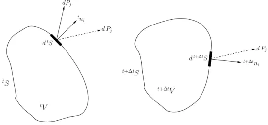
Figure 3.3: Total differential of a function.

f(x1+dx,y1+dy) ∼=f(x1,y1)+

∂f(x,y) ∂x

x1,y1

dx+∂f(x,y)

∂y

x1,y1

dy.

This concept can be extrapolated to a 3–D vector function as (see Figure 3.3b)

u∗_i =ui+

∂ui

∂t_x

1

dtx1+ ∂ui

∂t_x

2

dtx2+ ∂ui

∂t_x

3 dtx3

u∗_i −ui =

∂ui

∂t_x j

dtxj

(3.3)

where ∂ui

∂t_x

j =tui,j is known as the displacement gradient. This tensor can be

written as a 3×3 matrix, that is

tui,j =



    

∂u1

∂t_x

1

∂u1

∂t_x

2

∂u1

∂t_x

3

∂u2

∂t_x

1

∂u2

∂t_x

2

∂u2

∂t_x

3

∂u3

∂t_x

1

∂u3

∂t_x

2

∂u3

∂t_x

3



    

.

However, in order to get a general expression which relatesdt+∆t_x

(26)

the expressions stated in 3.1 are replaced into 3.3, which yields to

u∗_i −ui =

∂ui

∂t_x j

dtxj

dui =

∂ui

∂t_x j

dtxj

d(t+∆txi−txi) =

∂(t+∆t_x

i−txi)

∂t_x j

dtxj

dt+∆txi−dtxi =

∂t+∆t_x i

∂t_x j

dtxj −

∂t_x i

∂t_x j

dtxj

dt+∆txi−dtxi =

∂t+∆t_x i

∂t_x j

dtxj −δijdtxj

dt+∆txi−dtxi =

∂t+∆txi

∂t_x j

dtxj −dtxi

dt+∆txi =

∂t+∆txi

∂t_x j

dtxj;

hence,

dt+∆txi =tt+∆txi,jdtxj. (3.4)

The expressiont_t+∆txij is a second order tensor named in structural mechanics

as the deformation gradient. t_t+∆txi,j can be written in matrix form as

t+∆t t xi,j =



     

∂t+∆t_x

1

∂t_x

1

∂t+∆t_x

1

∂t_x

2

∂t+∆t_x

1

∂t_x

3

∂t+∆t_x

2

∂t_x

1

∂t+∆t_x

2

∂t_x

2

∂t+∆t_x

2

∂t_x

3

∂t+∆t_x

3

∂t_x

1

∂t+∆t_x

3

∂t_x

2

∂t+∆t_x

3

∂t_x

3



     

.

Both, the displacement gradienttui,j and the deformation gradienttt+∆txi,j

are taking place in configuration t+ ∆t; however, they are measured in con-figuration t.

“t_t+∆txi,j tensor includes rotation plus stretch effects which represents a

dis-advantage. Because constitutive equations employing it will have to be so con-structed that they will not predict a stress due to rigid body rotation”(Mal69)2_.

2_{For an enhancement of the displacement gradient concept consult references (Mal69),}

(27)

Appendix A deduces in matrix form how the expressions for the displacement gradient and the deformation gradient are obtained for a 3–D Cartesian sys-tem.

3.1.2 Green-Lagrange strain tensor

The mathematical definition of the Green-Lagrange strain tensor comes from the idea of measuring how much the length of a piece of material of differential size has changed when going from its initial configuration to its deformed configuration. Therefore, the measure obtained from the subtraction of the final and the initial length of vectorsdt+∆t_x

i and dtxi constitutes the basis to

define the Green-Lagrange strain.

The magnitudes of vectors dt+∆txi and dtxi can be quantified by their

Euclidean norm, that is

(kdt+∆txi k)2 =dt+∆txidt+∆txi and (kdtxi k)2 =dtxidtxi.

Next, using the Equation 3.4, the subtraction operation: length of dt+∆txi

minus length of dt_x

i can be developed as:

(kdt+∆txi k)2−(kdtxi k)2 =dt+∆txidt+∆txi −dtxidtxi

= ∂

t+∆t_x i

∂t_x j

dtxj

∂t+∆t_x i

∂t_x k

dtxk−dtxidtxi,

and using the expressions stated in 3.1, the following is obtained

dt+∆txidt+∆txi−dtxidtxi =

∂(ui +txi)

∂t_x j

dtxj

∂(ui+txi)

∂t_x k

dtxk−dtxidtxi

=h∂ui

∂t_x j

∂ui

∂t_x k

dtxjdtxk+

∂ui

∂t_x j

∂t_x i

∂t_x k

dtxjdtxk+

∂t_x i

∂t_x j

∂ui

∂t_x k

dtxjdtxk+

∂t_x i

∂t_x j

∂t_x i

∂t_x k

dtxjdtxk−

dtxidtxi

i

(28)

Now, multiplying by 1₂ in both sides of the equation 1

2

h

dt+∆txidt+∆txi−dtxidtxi

i

=1 2

h ∂u_i

∂t_x j

∂ui

∂t_x k

dtxjdtxk+

∂ui

∂t_x j

δikdtxjdtxk+

∂ui

∂t_x k

δijdtxjdtxk+δijδikdtxjdtxk−

dtxidtxi

i

=1 2

h ∂u_i

∂t_x j

∂ui

∂t_x k

dtxjdtxk+

∂uk

∂t_x j

dtxjdtxk+

∂uj

∂t_x k

dtxjdtxk+dtxidtxi−dtxidtxi

i

=1 2

h∂u_k

∂t_x j

+ ∂uj

∂t_x k

+ ∂ui

∂t_x j

∂ui

∂t_x k

i

| {z }

t+∆t t jk

dtxjdtxk.

Hence,

1 2

h

dt+∆txidt+∆txi−dtxidtxi

i

=dtxj tt+∆tjk dtxk,

wheret_t+∆tjk is the Green-Lagrange strain tensor taking place in configuration

t+ ∆t but measured in configuration t. It can also be easily deduced that

t+∆t t jk =

1 2

h

t+∆t

t xi,jtt+∆txi,k −δjk

i

= 1 2

h∂u_k

∂t_x j

+ ∂uj

∂t_x k

+ ∂ui

∂t_x j

∂ui

∂t_x k

i

. (3.5)

If the expression defined above is developed for a 3-D system, j = 1,2,3, and k = 1,2,3, each one of the terms of the Green-Lagrange tensor are ob-tained:

t+∆t t 11=

∂ u1 ∂t_x

1

+1 2

∂ u1 ∂t_x

1

2

+

∂ u2 ∂t_x

1

2

+

∂ u3 ∂t_x

1

2

t+∆t t 22=

∂ u2 ∂t_x

2

+1 2

∂ u1 ∂t_x

2

+

∂ u2 ∂t_x

2

+

∂ u3 ∂t_x

2

t+∆t t 33=

∂ u3 ∂t_x

3

+1 2

∂ u1 ∂t_x

3

2

+

∂ u2 ∂t_x

3

2

+

∂ u3 ∂t_x

3

(29)

t+∆t t 12=

1 2

∂ u2 ∂t_x

1

+ ∂ u1

∂t_x

2

+ ∂ u1

∂t_x

1 ∂ u1 ∂t_x

2

+ ∂ u2

∂t_x

1 ∂ u2 ∂t_x

2

+ ∂ u3

∂t_x

1 ∂ u3 ∂t_x

2

t+∆t t 13=

1 2

∂ u3 ∂t_x

1

+ ∂ u1

∂t_x

3

+ ∂ u1

∂t_x

1 ∂ u1 ∂t_x

3

+ ∂ u2

∂t_x

1 ∂ u2 ∂t_x

3

+ ∂ u3

∂t_x

1 ∂ u3 ∂t_x

3

t+∆t t 23=

1 2

∂ u3 ∂t_x

2

+ ∂ u2

∂t_x

3

+ ∂ u1

∂t_x

2 ∂ u1 ∂t_x

3

+ ∂ u2

∂t_x

2 ∂ u2 ∂t_x

3

+ ∂ u3

∂t_x

2 ∂ u3 ∂t_x

3

.

This strain measure t_t+∆tjk does not change under rigid-body rotations3, and

represents a complete finite strain tensor and not merely an approximation to it.

There is also an important deformation measure named right Cauchy-Green deformation tensor which is defined as

t+∆t

t Cij =tt+∆txi,k tt+∆txk,j, (3.6)

“ t_t+∆tCij is used to measure the stretch of a material fibber and the change

in angle between adjacent material fibres due to deformation”(Bat96). Indeed, the strain tensor t_t+∆tij can be written in terms of tt+∆tCij as4

2_tt+∆tij =tt+∆tCij −δij.

Both, t_t+∆tij and tt+∆tCij are positive-definite matrices, because they come

from the the evaluation of (k dt+∆txi k)2 and (k dtxi k)2 which are always

positive.

When the displacement gradient is finite, which means that it is not small compared to unity, it can also be demonstrated that5

t+∆t

t xk,p=tt+∆tRkqtt+∆tUqp

=t_t+∆tVkqtt+∆tRqp,

(3.7)

therefore,“a multiplicative decomposition into two tensors can be always achieved. One of which represents a rigid-body rotationt_t+∆tRkq, while the other is a

sym-metric positive-definite tensor t_t+∆tUqp or tt+∆tVkq”(Mal69).

3.1.3 Second Piola-Kirchhoff stress tensor

Looking back into chapter 1, and paying special attention in the way how the general equation of equilibrium for a 3–D structural object was deduced

3_{see (Bat96, pag. 518)}

(30)

(see Equation 1.4). It can be seen that the domain V represents the space of integration over which Expression 1.4 applies. Indeed, it was implicitly assumed that V stands for the current deformed configuration of the object, which means that V =t+∆tV.

In fact,“the stress tensor fieldτij is defined as function of the spatial

coordi-nates (Eulerian formulation). Therefore, a suitable strain measure to use with the Cauchy stress tensor would be one of the strain or deformation tensors of the Eulerian formulation in terms of the spatial position in the deformed con-figuration”(Mal69). But the Green-Lagrange strain recently defined with the intention of being used in a large displacement analysis, has been expressed in terms of the material points of the body (Lagrangian formulation). Hence, it becomes important to specify a stress measure as a function of the material coordinates, as well as a redefinition of the equilibrium equation of motion.

t_V

t+∆t_V

d Pj

d Pj t_n

i

dP˜j

t+∆t_S

dt+∆t_S

t+∆t_n i

dt_S

t_S

Figure 3.4: Force vectors for Piola-Kirchhoff stress definitions. Figure taken from (Mal69, pag. 221)

The Lagrangian stress tensor t_t+∆tTij or better called as the First

Piola-Kirchhoff stress tensor is defined through the expression

d Pj = (t+∆tni t+∆tτij)dt+∆tS = (tni tt+∆tTij)dtS,

where τij is the Cauchy stress tensor, and d Pj is the real force vector acting

over dt+∆t_S _{on the deformed configuration} t+∆t_V_{, see Figure 3.4. With the}

above expression, a new stress tensor measure t_t+∆tTij has been defined. This

(31)

non-deformed configuration; hence, it is defined in a material configuration scheme. But even t_t+∆tTij is very simple to define and leads to a simple form

of the equations of motion (equilibrium), it has the disadvantage of being not symmetric; in consequence, it cannot be used in constitutive equations with a symmetric strain tensor (Mal69).

The second Piola-Kirchhoff t_t+∆tSij comes up as a symmetric stress tensor

that can be used with the Green-Lagrange strain tensor through appropriate constitutive relation. “ t_t+∆tSij is formulated somewhat differently. Instead of

the actual force d Pj ondt+∆tS it gives a force dP˜j related to the forced Pj in

the same way that a material vector dtxi at tV is related by the deformation

to the corresponding spatial vector dt+∆t_x

i at t+∆tV. That is

dP˜i =

t+∆t t xi,j

−1

d Pj just as dtxi =

t+∆t t xi,j

−1

dt+∆txj

where dP˜i and dtS have been stretched and rotated the same amount relative

to the final positions d Pi and dt+∆tS respectively”(Mal69), then

dP˜j =

_t_+∆_t

t xj,q

−1 _t_+∆_t

ni t+∆tτiq

dt+∆tS

| {z }

d Pq

= tni tt+∆tSij

dtS. (3.8)

Now, in order to obtain an expression for the second Piola-Kirchhoff stress in terms of the Cauchy stress, it is necessary to use the Nanson’s formula6 _which

says that,

t+∆t_ρt+∆t_n

jdt+∆tS=tρtni

_t_+∆_t

t xi,j

−1

dtS.

Replacing this formula into 3.8 yields to

t_n

i tt+∆tSij

dtS =t_t+∆txj,q

−1 _t_+∆_t

np t+∆tτpq

dt+∆tS

t_n

i tt+∆tSij

dtS =t+∆t t xj,q

−1 t_ρ

t+∆t_ρ t_n

k

t+∆t t xk,p

−1 d

t_S

dt+∆t_S

t+∆t_τ

pqdt+∆tS t_n

i tt+∆tSij

=

t_ρ t+∆t_ρ

t_n

ktt+∆txk,pt+∆tτpqtt+∆txj,q.

Finally, “for arbitrary unit vector t_ˆ_{n, because this relationship must hold for}

any surface area and also any interior surface area that could be created by a cut in the body. Hence t_n

i is arbitrary and can be chosen to be in succession

equal to the unit coordinate vectors”(Mal69), then

t+∆t t Sij =

t_ρ t+∆t_ρ

t

t+∆txi,p t+∆tτpq tt+∆txj,q. (3.9)

(32)

This is the expression usually used in large displacement structural mechanics to relate Cauchy stresses with the second Piola-Kirchoff stress tensor.

3.2 Non-linear equations of motion

The principle of virtual displacements (Equation 1.2) deduced in chapter 1 is expressed in terms of the spatial coordinates (Eulerian formulation) at time

t+ ∆t. In other words, it is applicable to the current deformed configuration of the object. Therefore, Equation 1.2 can be rewritten as

Z

t+∆t_V

t+∆t_τ

ijδ(t+∆teij)dt+∆tV =

Z

t+∆t_V

t+∆t_fB i δ

t+∆t_u i

dt+∆tV

+

Z

t+∆t_S f

t+∆t

fSf

i δ

t+∆t

uSf

i

dt+∆tS

(3.10)

In structural mechanics, a Lagrangian formulation is usually preferred instead of the Eulerian formulation. This happens because the volume of the object being analysed is not known at time t+ ∆t, and also because it is assumed that the body would return to its natural state when it is unloaded (Mal69).

It is then necessary to rewrite Equation 3.10 using a Lagrangian formula-tion. In section 3.1.3 it was shown that the Cauchy stress tensort+∆t_τ

ij can be

expressed in terms of the second Piola-Kirchhoff stress tensor t_t+∆tSij, which

is already written in terms of the material coordinates. However, it is still in-dispensable to transform the termδt+∆teij to be able to express the left hand

side of Equation 3.10 in Lagrangian form.

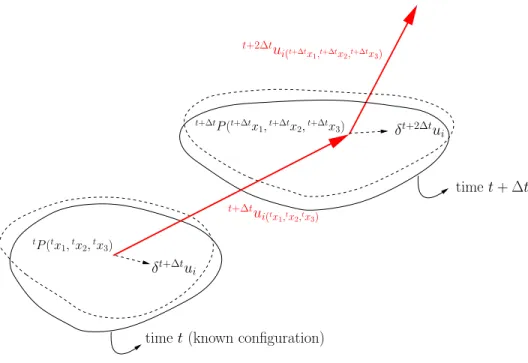
For this purpose, it is precise to consider both a body in its deformed configuration (timet+ ∆t), and in its previous known configuration at time t

(timet can be a deformed previous calculated configuration t_V _{or the original}

undeformed configuration 0_V_{), see Figure 3.5. A virtual displacement field} δt+2∆tui is applied. This field is a function of the spatial coordinatest+∆t(see

Figure 3.5), and can also be thought as a variation on the displacement field

t+∆t_u

i. Hence, it is conceivable to assume thatδt+2∆tui ∼=δt+∆tui. Moreover, a

variation fieldt+∆tui will cause a variation on the small stress tensorδt+∆teij,

where

t+∆teij =

1 2

∂t+2∆tui

∂t+∆t_x j

+ ∂

t+2∆t_u j

∂t+∆t_x i

= 1 2

t+2∆t t+∆t ui,j +

t+2∆t t+∆t uj,i

(33)

3.2. Non-linear equations of motion 33

timet+ ∆t

timet(known configuration)

t+∆t_u

i(t_x₁_,t_x₂_,t_x₃₎

t_P₍t_x

1,tx2,tx3)

δt+∆tui

δt+2∆t_u i

t+2∆t_u

i(t+∆t_x₁_,t+∆t_x₂_,t+∆t_x₃₎

t+∆t_P₍t+∆t_x

1,t+∆tx2,t+∆tx3)

Figure 3.5: Body at time t+ ∆t subjected to virtual displacement field given byδt+∆tui. Figure taken from (Bat96, pag. 514)

and t+2∆t_u

i is a function of the spatial coordinates at time t+ ∆t. That is, t+2∆t_u

i(t+∆t_x

1,t+∆tx2,t+∆tx3). Besides

t+∆t t =

1 2

h

t+∆t

t xk,itt+∆txk,j−δij

i

,

and

δt_t+∆t= 1 2

h

δ_tt+∆txk,i tt+∆txk,j+tt+∆txk,i δtt+∆txk,j−δ(δij)

i

, (3.12)

where δ(δij) = 0 because it represents the variation of the delta Kronecker

δij which is a constant tensor. Now, it is necessary to find an expression for

δt_t+∆txi,j

δt_t+∆txi,j =

∂δt+∆txi

∂t_x j

= ∂δ(

t_x

i+t+∆tui)

∂t_x j

=δ(δij) +

∂δ(t+∆tui)

∂t_x j

= ∂δ(

t+∆t_u i)

∂t_x j

;

but δt+2∆t_u

i ∼=δt+∆tui, then

δt_t+∆txi,j =

∂δ(t+∆tui)

∂t_x j

∼

= ∂δ(

t+2∆t_u i)

∂t_x j

(34)

Finally,

δt_t+∆txi,j =

∂δ(t+2∆t_u i)

∂t+∆t_x p

∂t_x j

=

t+2∆t t+∆t ui,p

t

t+∆txp,j

. (3.13)

Replacing this expression into Equation 3.12,

δt_t+∆tij =

1 2

h

δt_t+2∆_+∆_ttuk,p

t+∆t

t xp,itt+∆txk,j+tt+∆txk,i

δt_t+2∆_+∆_ttuk,n

t+∆t t xn,j

| {z }

changing indexkbyp

i

= 1 2

h

t+∆t t xp,i

t+∆t

t xk,j+tt+∆txp,i

δt_t+2∆_+∆_ttup,n

t+∆t t xn,j

| {z }

changing indexnbyk

i

= 1 2

h

t+∆t t xp,i

t+∆t

t xk,j+tt+∆txp,i

δt_t+2∆_+∆_ttup,k

t+∆t t xk,j

i

=t_t+∆txp,i

h1

2

δt_t+2∆_+∆_ttuk,p+δt_t+2∆_+∆_ttup,k

i

t+∆t t xk,j,

and according to Equation 3.11, it can be easily seen that

δt_t+∆tij =tt+∆txp,i

h

δt+∆tekp

i

t+∆t

t xk,j. (3.14)

Now, the left side of Equation 3.10 can be transformed into

Z

t+∆t_V

t+∆t_τ

ijδt+∆teijdt+∆tV =

Z

t+∆t_V

t+∆t_ρ t_ρ

t+∆t

t xi,ptt+∆tSpqtt+∆txj,q

t

t+∆txn,i

h

δt_t_+∆_tmn

i

t

t+∆txm,j

dt+∆tV.

And because

t+∆t

t xi,p tt+∆txn,i=δnp, and tt+∆txj,q tt+∆txm,j =δmq;

thus

Z

t+∆t_V

t+∆t

τijδt+∆teij dt+∆tV =

Z

t+∆t_V

t+∆t_ρ

t_ρ δnpδmq t+∆t

t Spqδtt+∆tmn

dt+∆tV

=

Z

t_V

t+∆t

t Spqδtt+∆tpqdtV

wheret+∆tρ dt+∆tV =tρ dtV. In this way,

Z

t_V

t+∆t

t Spqδtt+∆tpqdtV =

Z

t+∆t_V

t+∆t_fB i δ

t+∆t_u

idt+∆tV

+

Z

t+∆t_S f

t+∆t_fSf

i δ

t+∆t_uSf

i d t+∆t_S.

(35)

3.2. Non-linear equations of motion 35

This result is used for the development of the two general continuum mechanics incremental formulations of nonlinear problems: Total Lagrangian (TL) and Updated Lagrangian (UL). In the TL formulation all static and kinematic variables are referred to the initial configuration at time 0. Whereas in the UL formulation all the static and kinematic variables are referred to the last calculated configuration at time t (Bat96).

The result found in 3.15 is referred to configuration at time t, but instead, configuration at time 0 could be chosen. This means that any possible con-figuration between time 0 and t can be used to refer all the variables in 3.15. Therefore, it is also feasible to state that

Z

t+∆t_V

t+∆t

τijδt+∆teijdt+∆tV =

Z

0_V

t+∆t

0 Spqδt0+∆tpqd0V, (3.16)

and

Z

0_V

t+∆t

0 Spqδt0+∆tpqd0V =

Z

t+∆t_V

t+∆t_fB

i δt+∆tuidt+∆tV

+

Z

t+∆t_S f

t+∆t_fSf

i δ

t+∆t_uSf

i d t+∆t_S,

(3.17)

which represents the general expression used for the TL formulation.

The right hand side of equations 3.15 and 3.17 is still written in terms of configuration at time t+ ∆t. To overcome this problem and for simplicity it will be assumed that the loading is deformation-independent. This implies that the load does not change its direction and magnitude as a function of the displacement. This specific type of loading is typically used to model concentrated loads which in reality are forces acting over a small surface area. The deformation-independent assumption allows to state that the load will be the same during the whole incremental process and the integration will be carried out over 0_V_{. Hence}

t+∆t_R ₌

Z

t+∆t_V

t+∆t_fB i δ

t+∆t_u

idt+∆tV +

Z

t+∆t_S f

t+∆t_fSf

i δ

t+∆t_uSf

i d t+∆t_S

=

Z

0_V

0_fB

i δ0uid0V +

Z

0_S

f

0_fSf

i δ

0_uSf

i d

0_S.

(3.18)

(36)

which in general cannot be solve directly. Therefore,“an approximate solution can be obtained by referring all variables to a previously calculated known equi-librium configuration and linearising the resulting equation. This solution can be improved by an iteration process”(Bat96). Hereafter, the solution at time

t will be considered as the last calculated equilibrium configuration. Between time 0 and time t there is the whole path of time steps previously calculated by the iteration procedure. However, for the TL and UL formulations, only configurations at time 0 andt(not the whole path of time steps between them) are important. This fact occurs because all the static and kinematic variables are referred to times 0 and t.

3.3 Linearisation of the principle of virtual

dis-placements.

Total Lagrangian

Formula-tion

In this report, the TL formulation has been chosen instead of the UL formu-lation. There is no apparent reason to take this decision; indeed, it does not matter what formulation is chosen“if in the numerical solution the appropriate constitutive tensors are employed, identical results are obtained”(Bat96).

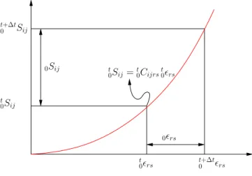
First, it is appropriate to get the incremental decomposition for the second Piola-Kirchhoff stresses and the Green-Lagrange strain: According to Figure

t

0rs

0Sij

t+∆t

0 rs

0rs t

0Sij t+∆t

0 Sij

t

0Sij =t0Cijrst0rs

(37)

3.3. Total Lagrangian Formulation 37

3.6, it can be appreciated that

t+∆t

0 Sij =t0Sij +0Sij (3.19)

t+∆t

0 rs =t0rs+0rs, t

0Cijrs represents a four order tensor which relates the second Piola-Kirchhoff

stresses with the Green-Lagrange strains. In this particular case the t₀Cijrs

tensor takes place at time t but is measured in configuration at time 0. It is important to remember that t₀Cijrs can be linear or non-linear. Indeed,

the effectiveness of the iterative procedure and, whether a large or a small strain formulation is considered, depends on the use of appropriate stress-strain relationships. Note that the four order tensor t

0Cijrs is different to the

right Cauchy-Green deformation tensor t₀Cij, which is a second order tensor.

Equation 3.5 can be written as

t+∆t

0 ij =

1 2

∂t+∆t_u i

∂0_x

j

+ ∂

t+∆t_u j

∂0_x

i

+∂

t+∆t_u k

∂0_x

i

∂t+∆t_u k

∂0_x

j

,

where t+∆t_u

i =tui+ui, then

t+∆t

0 ij =

1 2

∂tui

∂0_x

j

+ ∂ui

∂0_x

j

+∂

t_u j

∂0_x

i

+ ∂uj

∂0_x

i

+

∂tuk

∂0_x

i

+ ∂uk

∂0_x

i

∂tuk

∂0_x

j

+ ∂uk

∂0_x

j

= 1 2

h∂tu_i

∂0_x

j

+ ∂ui

∂0_x

j

+∂

t_u j

∂0_x

i

+ ∂uj

∂0_x

i

+ ∂

t_u k

∂0_x

i

∂t_u k

∂0_x

j

+

∂t_u k

∂0_x

i

∂uk

∂0_x

j

+ ∂uk

∂0_x

i

∂t_u k

∂0_x

j

+ ∂uk

∂0_x

i

∂uk

∂0_x

j

i

= 1 2

∂tui

∂0_x

j

+∂

t_u j

∂0_x

i

+ ∂

t_u k

∂0_x

i

∂tuk

∂0_x

j

| {z }

t

0ij

+

1 2

∂ui

∂0_x

j

∂uj

∂0_x

i

+ ∂

t_u k

∂0_x

i

∂uk

∂0_x

j

+ ∂uk

∂0_x

i

∂t_u k

∂0_x

j

| {z }

0eij

+1 2

∂uk

∂0_x

i

∂uk

∂0_x

j

| {z }

0ηij

.

Thus

t+∆t

0 ij =t0ij +0eij +0ηij

| {z }

0ij

;

therefore, it can be said that

(38)

but δt₀ij = 0 because the variation is taken about the configuration at time

t+ ∆t.

Replacing equations 3.19 and 3.20 into the principle of virtual displace-ments (Equation 3.17), the following expression is obtained

Z

0_V

t+∆t

0 Sijδt0+∆tijd0V =t+∆tR

Z

0_V

t

0Sij +0Sij δ0eij+δ0ηij

| {z }

δ0ij

d0V =t+∆tR

Z

0_V

t

0Sijδ0eij +t0Sijδ0ηij +0Sijδ0ij

d0V =t+∆tR

Z

0_V

0Sijδ0ijd0V

| {z }

term 1

+

Z

0_V

t

0Sijδ0ηijd0V

| {z }

term 2

=t+∆tR

| {z }

term 3

−

Z

0_V

t

0Sijδ0eij

| {z }

term 4 .

Terms 2, 3, and 4 are linear in the incremental displacements ui, but term 1

is highly nonlinear. The linearity of terms 2, 3, and 4, with respect toui will

be evident once the discrete finite element equations are assembled. Instead, term 1 has to be linearised, for that porpuse a Taylor series of expansion up to a first order of approximation is used. That is,

t+∆t

0 Sij =t0Sij+

∂t

0Sij

∂t

0rs

0rs t+∆t

0 Sij −t0Sij =0Sij =t0Cijrs0rs,

using this approximation, term 1 is transformed into

Z

0_V

0Sijδ0ijd0V =

Z

0_V

t

0Cijrs0rs

δ0ijd0V

=

Z

0_V

t

0Cijrs

0ers+0 ηrs

|{z}

neglect

δ0eij +0 ηij

|{z}

neglect

d0V

=

Z

0_V

t

0Cijrs0ersδ0eijd0V.

The linearisation procedure explained here constitutes an enhanced deduction of the one published by reference (Bat96, pag. 525).

Finally, the linearised principle of virtual displacements in a TL formulation can be written as

Z

0_V

t

0Cijrs0ersδ0eijd0V +

Z

0_V

t

0Sijδ0ηijd0V =t+∆tR−

Z

0_V

t

(39)

3.3. Total Lagrangian Formulation 39

this expression is used directly in the Finite Element formulation for large displacements. The above equation can be written in matrix notation as

δuˆT

Z

0_V

t

0B

T L

t

0C

t

0BL d0V +

Z

0_V

t

0B

T N L

t

0S

t

0BN L d0V

ˆ

u=

δuˆTt+∆tR−

Z

0_V

t

0B

T L

t

0Sd 0_V_,

and following the same procedure explained in section 2.1 yields to,

t

0KL+t0KN L

ˆ

u=t+∆tR−t₀F. (3.22)

In the next chapters, matrices t

0KL, t0KN L, and vectors t+∆tR, and t0F will be

deduced for several types of elements.

Once the linear system of equations 3.22 is solved, it is precise to find how much difference there exists between the internal virtual work and the external virtual work, and continue with an iterative procedure until this difference tends to zero. The internal virtual work can be calculated with the state variables calculated by the system of finite equations, and the external virtual work is given by t+∆t_R_.7

(40)

(41)

Chapter 4 Bar or Truss Elements

When begining with the study of the underlying theory used by the Finite Element Method, usually bars or truss elements are chosen as the first type of elements to be analysed. These elements are chosen because they are easy to define from the structural point of view; furthermore, the Finite Element equations can be mathematically deduced in a simple and understandable way. A truss element is defined as a structural part, which is capable of supporting loads only in the direction normal to its cross-sectional area. Therefore, the strains and the stresses can only be transmitted in that direction. It is also important to remark that the strains and the stresses are considered to be constant over the cross-sectional area of the element.

4.1 Bars under the small displacements

hy-pothesis

Considering only small displacements and small deformations for a two-node bar element with only one degree of freedom per node, and with constant cross-sectional area, it can be easily deduced that its stiffness matrix is given by

(m)_K ₌ E A L

1 −1

−1 1

, (4.1)

where E is the linear-elastic modulus of the material, A is the value of the cross-sectional area, and L is the length of the bar. Hereafter this point, the superscript (m), which denotes the m-th element of the assemblage, will be ommited; this is done because henceforward only the FEM equations for single non-assembled elements will be stated.

(42)

42 Chapter 4. Bar or Truss Elements

To be able to arrive to the stiffness matrix 4.1, the Finite Element equa-tions can be proposed in any convenient reference system. It is clear that if an inconvenient reference system is chosen, some mathematical problems in the deduction process might be obtained, but eventually, because of the Frame Indifference Principle1 _{the same results must be achieved. The Frame}

Indiffer-ence Principle states that the frame of referIndiffer-ence is only a mathematical artifice and it does not have any physical meaning. Therefore, it does not matter which frame of reference is chosen, the physical response of the structure analysed cannot be affected.

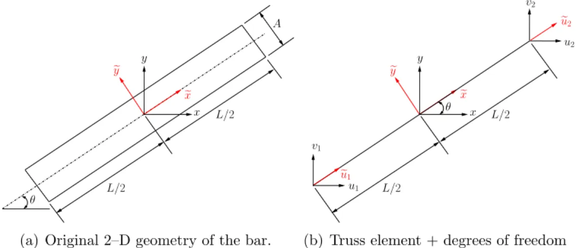
To aim towards the understanding of this principle, the FEM equations for a truss element will be stated in two different systems of reference; of course, the final results found must be similar. The problem to be solved can be defined as: A unidimensional truss element is located in the x−y Cartesian plane, and it has been rotated aθ angle with respect to the xaxis. The element has constant cross-sectional areaA, a total length L, and its modulus of elasticity is E; see Figure 4.1a. Find the stiffness matrix of the element, stating the strain and the stress tensors both in a x−y global Cartesian system, and in ax_e−y_elocal system.

L/2

A

θ

e

y y

e

x x

(a) Original 2–D geometry of the bar.

y

L/2

θ

v2

u2

e

u1 e

y

e

u2

u1

v1

e

x x

(b) Truss element + degrees of freedom

Figure 4.1: Bar or truss element

First, a convenient local reference system x_e−y_ewhich coincides with the principal axes of the element is chosen, see Figure 4.1. It is also important to remember that a truss element can only support tension or compression loads. For that reason, in the local system of reference, only degrees of freedom _eu1