TítuloA Finite element formulation for the resolution of the unsteady incompressible viscous flow for low Reynolds numbers

(1)

Preprint of the paper

"A Finite Element formulation for the resolution of the unsteady incompressible viscous flow for low Reynolds numbers"

P. Vellando, J. Puertas, J. Bonillo, J. Fe (1999)

CD Proceedings of the XXVIII Congress of the IAHR (International asociation for hydraulic research).

(2)

A FINITE ELEMENT FORMULATION FOR THE RESOLUTION OF THE

UNSTEADY INCOMPRESSIBLE VISCOUS FLOW FOR LOW

REYNOLDS NUMBERS.

*P. VELLANDO, **J. PUERTAS, **J. BONILLO, *J. FE.

ETS. de Ingenieros de Caminos, Canales y Puertos.*Dpto. de Métodos Matemáticos y de Representación. **Dpto. de Tecnología de la Construcción.

Universidad de La Coruña. Campus de Elviña. 15192 La Coruña, Spain. Tel: (34) 981 167000, fax: (34) 981 167170. E-mail: vellando@iccp.udc.es

ABSTRACT

The following paper shows a Finite Element formulation for the resolution of the – local and convective acceleration terms including- Navier-Stokes equations, which gives analytical response to the problem of viscous, incompressible, unsteady flows. The integration of the resulting non-linear system of first order ordinary differential equations, is made upon a successive approximation algorithm together with an implicit backward time integrating scheme. The interpolation of the spatial domain is made in terms of a Q1/P0 pair (bilinear velocity-constant pressure). The usage of a Bubnov Galerkin formulation in the process of obtaining a weak form implies that flows of a certain velocity need the employment of a very refined spatial mesh so as to avoid numerical instability. For high Reynolds numbers the convection term becomes predominant compared to the diffussion term and a different algorithm (SPGU, GLS), should be introduced. Finally the developed program is checked over some of the most commonly used flow tests and its results on velocity and pressure are shown.

GOVERNING EQUATIONS

The unsteady incompressible Navier-Stokes equations are given by:

(

u

)

u u f

u₊ _⋅_∇ ₋ _∆ ₊_∇ ₌

p

t ν

∂ ∂

in Ω

∇ ⋅ =u 0 in Ω (1.1)

for 0≤t ≤T , (whereT is a specified time), together with the initial and boundary conditions:

( )

x, u

( )

x

u 0 = 0 in Ω

u=g on ∂Ω ×

(

0,T

)

(1.2)

where u is the velocity, p is the pressure, t is the time, ν is the cinematic viscosity, f is the body force per unit mass and ∇,∆,are the gradient and laplacian tensor operators. The problem consists in finding u∈H₀1 and p∈S₀1in a time-space domain

Ωx(0,T).

(3)

Let V be the subspace of D(Ω) satisfying the incompressibility constraint:

( )

{

∈ Ω ∇⋅ =0

}

= u D : u

V , let H be the closure of V in 1

( )

Ω 0

H . If Ω is sufficiently well behaved then H =

{

u∈

(

H1

( )

Ω

)

n :∇⋅u=0in Ω

}

.

If we apply the weighted-residual argument by taking the scalar product of the momentum equation times an arbitrary test function v satisfying ∇⋅v=0, that is for

V ∈ v ,

(

)

_∫

∫

Ω Ω Ω Ω Ω Ω ⋅ = Ω ⋅ ∇ + Ω ⋅ ∆ − Ω ⋅ ∇ ⋅ + Ω ⋅ ∂ ∂ d d p d d d

t v u u v u v v f v

u _ν

(2.1)

Applying the divergence theorem and taking into account that ∇⋅v=0 in Ω, we arrive to:

(

)

_∫

∫

Ω Ω Ω Ω Ω Ω ⋅ = Ω ⋅ ∇ − Ω ∇ ∇ + Ω ⋅ ∇ ⋅ + Ω

⋅ d d p d

t vd u u v u: v vd f v

u _ν

∂ ∂

(2.2)

for all admissible functions v∈V .

Even with ∇⋅v=0 in Ω, we will maintain the pressure term so as to be able to use a mixed formulation rather than the penalized one. This allows us to keep as variables the pressure unknowns.Although it produces a certain increase in computational cost, the penalty parameter formulation is known to be the cause of loss of accuracy for small values and for holding up the convergence of the solution for too large ones. In the same way, making the scalar product of the continuity equation with an arbitrary test function q∈L2

( )

Ω /R=P

, the weak expression turns into:

(

)

∫

Ω

Ω ⋅

∇ u qd (2.3)

The velocity and pressure fields may be approximated now as piecewise polynomials on the discretization by (Q1/P0) Lagrange-Type elements, so they are expressed in terms of the trial functions, φ_n

( )

x , χ_m

( )

x .

( )

x u

( )

x u

( )

x

u n

N

n n

h

∑

φ

=

= ≈

1

( )

x

( )

x m

( )

x

M

m m

h p

p

∑

χ

=

= ≈

1

(2.4)

Replacing (2.4) into (2.2) and (2.3):

(

)

_∫

∫

Ω Ω Ω Ω Ω Ω ⋅ = Ω ⋅ ∇ − Ω ∇ ∇ + Ω ⋅ ∇ ⋅ + Ω

⋅ d d p d d

t h h h h h h h h h

h

d u u v u : v v f v

v u ν ∂ ∂ (2.5)

(

)

∫

Ω Ω ⋅

∇ u_h q_h d (2.6)

For all admissible test functions h h ∈V

v and h

h P

q ∈ .

Introducing the expansions for uh,ph, and integrating, the following non-linear

(4)

( )

u Au Bp F C

u

M & + +ν − =

0 u

BT = (2.7)

In expanded matrix form:

( )

( ) ( )

         =                     + +                     0 F F u u 0 B B B Aˆ 0 B 0 Aˆ u C u u 0 0 0 0 Mˆ 0 0 0 Mˆ 2 1 2 1 1 1 p

p x T y T

y x ν ν & & & (2.8) where:

( )

=

_∫

_Ω + = h dx y y x x

Ars r s r s

∂ ∂φ ∂ ∂φ ∂ ∂φ ∂ ∂φ ˆ

Aˆ

( )

∫

Ω Ω = = h d s r rs

Mˆ φ φ

Mˆ

( )

Bx _rtx r

t B x dx h = =

∫

∂φ ∂ χ

Ω B

( )

y rt y r t B y dx h = =

∫

∂φ ∂ χ Ω

F_rx f _rdx

h

=

∫

_Ω 1φ =

∫

_Ω

h

dx f

F_ry ₂φ_r (2.9)

In order to turn equation (2.8) into a linear system of equations we are going to approximate the non-linear term C

( )

u , by an iterative scheme known as successive-approximation:

( ) ( )

_∫

(

)

Ω −

− = ⋅∇ ⋅ Ω

≈ _k _k k_h k_h _h d

k

1

1 u u u v

u c u

c (2.10)

Thus (2.7) is written:

k k k

k

k Cu Au Bp F

u

M & + +ν − =

0 u

BT *_k = (2.11)

Where C is:

          = 0 0 0 0 C 0 0 0 C

C C

(

)

(

)

dx

y v x u i j k k j k k ij h φ φ φ φ φ

∫

Ω      ∂ ∂ + ∂ ∂ = (2.12)

Finally, the time integration based on an implicit backward scheme, results in the following non-differential linear system:

1 1 1 1 1 + + + + + ₊ ₊ ₋ ₌     ∆ − n n n n n n

t Cu Au Bp F

u u

M ν (2.13)

0 u BT _n₊₁ =

(5)

DISCRETIZATION

The Q1/P0 pair means a quadratic first order approximation for the velocity field and a constant pressure approximation for each basic element. The shape functions for the velocity field Ni are expressed in terms of the local coordinates η,ξ.

(

)(

)

(

)(

)

(

)(

)

(

1

)(

1

)

4 1 1 1 4 1 1 1 4 1 1 1 4 1 4 3 2 1 + − − = − − = − + − = + + = η ξ η ξ η ξ η ξ N N N N , , (3.1)

The derivatives of the form functions with respect to the global axis coordinates must be calculated so as to be able to constitute the basic matrices, the change of coordinates leads to:

( )

∂η ∂ ∂ξ ∂ ∂η ∂ ∂η ∂ ∂ξ ∂ η ξ ∂ ∂ ∂ξ ∂ ∂ξ ∂ ∂η ∂ ∂η ∂ ∂ξ ∂ η ξ ∂ ∂ e i K K k k i k k i i e i K K k k i k k i i N N x N N x N J y N N N y N N y N J x N =    ₋ ₊ = =     ₋ =

∑

= = = = 4 1 4 1 4 1 4 1 1 1 , , (3.2)

Combining the former expressions, the matrices M, A, Bx, By, C may be now expressed in terms of the derivatives with respect to the local axis coordinates. So, the matrix Bx (for instance) being:

( )

∂ξ ξ η ∂ ∂η ∂ ∂η ∂ ∂ξ ∂ ∂ξ η ξ ∂ ∂η η ξ ∂ ∂η η ξ ∂ ∂ξ η ξ ∂ η

ξ d d

N x N N x N N y N N y N

J K K

k k i k k i K K k k i k k i 1 4 1 4 1 4 1 4 1    ₋ ₊     ₋ =

_∫∫

∑

= = = = , , , , ,

B_x (3.3)

The integration of expression (3.3) and that of the other matrices will be carried out, following a numerical 4-point two-dimensional Gauss integration, where the Gauss points are in

(

±0.5773,±0.5773

)

, and the weighting function H=1.

( )

(

)

∫∫

∑∑

= = = = 2 1 2 1 i j j i j iH F

H d

d F

I ξ,η ξ η ξ ,η (3.4)

NUMERICAL EXAMPLES

A FORTRAN code has been developed making use of the previously explained formulation. The program has been checked with the well known backward step and driven cavity flow tests and the results for velocity and pressure unknowns are shown bellow

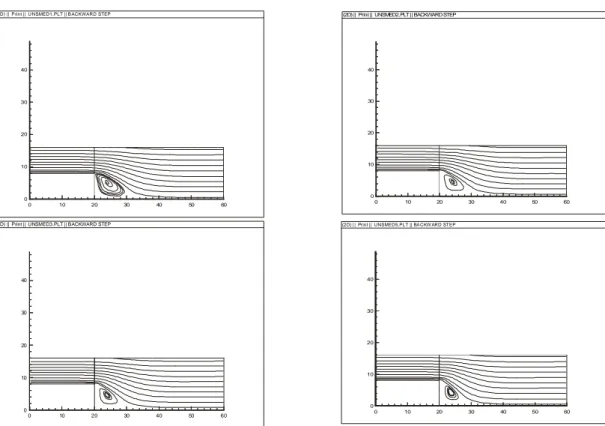
The following figure shows the evolution in time of the behaviour of the streamlines for the backward step problem in which the eddy takes form for flow decreasing boundary conditions.

(6)

0 10 20 30 40 50 60 0

10 20 30 40

(2D) || P rint || U NSMED1.PLT | | B ACKWARD STEP

0 10 20 30 40 50 60

0 10 20 30 40

(2D) || Print || UNSMED2.PLT || BACKWARD STEP

0 10 20 30 40 50 60

0 10 20 30 40

(2D) || Print || UNSMED3.PLT || BACKWARD STEP

0 10 20 30 40 50 60

0 10 20 30 40

(2D) | | Print || UNSMED5.PLT || BA CKW ARD STEP

Fig 1. Backward step streamlines varying in time.

The results of the velocity field, both for the backward step and cavity flow are plotted bellow

0 10 20 30 40 50 60

0 10 20 30 40

(2D) || Print || UNSMED1.PLT || BACK WARD STEP

0 10 20 30 40

0 5 10 15 20 25 30 35 40

(2D) || P rint || GRAZ201.PLT || ca vity flow

Fig 2. Velocity fields.

(7)

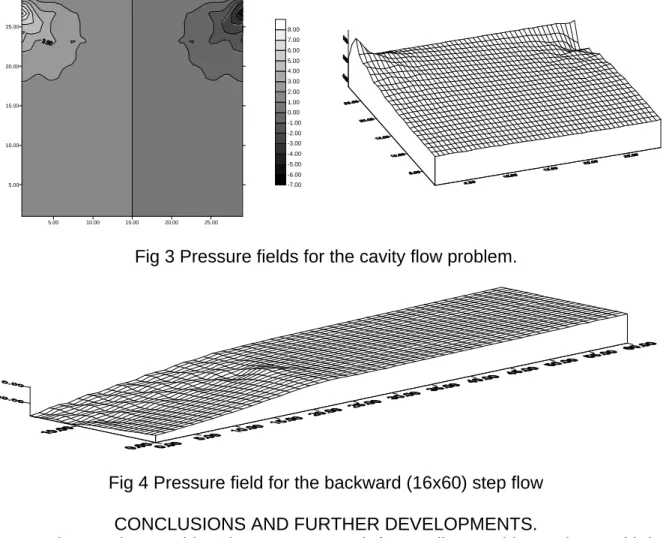
5.00 10.00 15.00 20.00 25.00 5.00

10.00 15.00 20.00 25.00

-7.00 -6.00 -5.00 -4.00 -3.00 -2.00 -1.00 0.00 1.00 2.00 3.00 4.00 5.00 6.00 7.00 8.00

Fig 3 Pressure fields for the cavity flow problem.

Fig 4 Pressure field for the backward (16x60) step flow

CONCLUSIONS AND FURTHER DEVELOPMENTS.

The results may be considered accurate enough for small Reynolds numbers, with its magnitude being a function of the mesh grade of refinement. Once the Reynolds number becomes of considerable magnitude (and so the convective term gets bigger compared with the diffusive term), the upwinding Petrov Galerking formulation together with the inclusion of an artificial streamline diffusion term (SUPG), should provide a computationaly speaking inexpensive and convenient approach. Next, a turbulence-considering scheme and a pattern being able to model transitions in flow, would be implemented.

REFERENCES

[1] I Christie, O. F. Griffith, A. R. Mitchel, O. C. Zienkiewicz. Finite element methods for second-order differential equations with significant first order derivatives. Int. J. Numer. Methods Engrg. 10 (1976) 1389-1396.

[2] A. N. Brooks, T. J. R. Hughes, Streamline upwind/Petrov-Galerkin formulation for convection dominated flows with particular emphasis on the incompressible Navier-Stokes equation, Comput. Methods Appl. Mech. Engrg. 32 (1982) 199-259.

[3] G. F. Carey, J. T. Oden, Finite Elements, Prentice Hall, (1983).

[4] , T. J. R. Hughes, M. Mallet, A. Mizukami, A new finite element formulation for computational fluid dynamics: II Beyod SUPG, Comput. Methods Appl. Mech. Engrg. 54 (1986) 341-355.

[5] M. D. Gunzburger, “Finite Element Methods for Viscous Incompressible Flows, AcademicPress,(1989).

(8)

[7] , T. J. R. Hughes, L. P. Franca, G. M. Hulbert. A new finite element formulation for computational fluid dynamics: VIII The Galerkin Least-Squares Method for advective-diffusive equations. Comput. Methods Appl. Mech. Engrg. 73 (1989) 173-189.

[8] O. C. Zienkiewicz, R. L. Taylor, The Finite Element Method, Mc Graw Hill, (1991). [9] L. P. Franca, S. L. Frey Stabilized finite element methods: II The incompressible Navier-Stokes equation. Comput. Methods Appl. Mech. Engrg. 99 (1992) 209-233. [10] S. K. Hannani, M. Stanislas, P. Dupont, Incompressible Navier-Stokes computations with SUPG and GLS formulations-A comparison study. Comput. Methods Appl. Mech. Engrg. 124 (1995) 153-170.