Comparison of dynamic effects of
high-speed traffic load on ballasted
track using a simplified two-dimensional
and full three-dimensional model
K Nguyen, JM Goicolea and F Galbado
´ n
Abstract
The vertical dynamic actions transmitted by railway vehicles to the ballasted track infrastructure are evaluated taking into account models with different degrees of detail. In particular, this matter has been studied from a two-dimensional finite-element model to a fully coupled three-dimensional multibody finite-finite-element model. The vehicle and track are coupled via a nonlinear Hertz contact mechanism. The method of Lagrange multipliers is used for the contact constraint enforcement between the wheel and rail. Distributed elevation irregularities are generated based on power spectral density distributions, which are taken into account for the interaction. Due to the contact nonlinearities, the numerical simulations are performed in the time domain, using a direct integration method for the transient problem. The results obtained include contact forces, forces transmitted to the infrastructure (sleeper) by railpads, and envelopes of relevant results for several track irregularities and speed ranges. The main contribution of this work is to identify and discuss coincidences and differences between discrete two-dimensional models and continuum three-dimensional models, as well to assess the validity of evaluating the dynamic loading on the track with simplified two-dimensional models.
Keywords
Dynamic response, infinite element, track irregularities, vehicle–track interaction, wheel–rail contact
Date received: 25 April 2012; accepted: 3 October 2012
Introduction
The advent and success of high-speed railways and the increasing demand for sustainable development is enabling a comeback of railway transport, which is increasing the share in passenger traffic and perhaps also freight traffic. This is a clear trend in Europe and Asia. An implication of this development is the requirement for new standards and regulations, which, among other objectives, must provide criteria for safety and functionality of new or existing railway infrastructure.1–3
The evaluation of the dynamic response of railway track subjected to high-speed loading represents one of the main structural issues for the design of high-speed railway structures. The dynamic behaviour of the railway track structure induced by the traffic is influenced by the interaction between the train and the complete track structure, as well as by the dynamic configuration of vehicles. As the operating speed of train becomes higher and reaches 350 km/h or more, accuracy in the analysis of the vehicle–track interaction becomes an important factor to be con-sidered in railway track design. An important number of research works on this subject have
This work focuses on issues related to the mechan-ical actions on the track structure, specifically vertmechan-ical dynamic loads. The aim of the present work is developing different vehicle–track interaction models, as well as obtaining and comparing the dynamic response on the track structures obtained in these models: the contact force between the wheel and rail, the force transmitted to the railpads, the vibration in the rail, and making recommendations for efficient and rational modelling. For this purpose, a simplified 2D and a full 3D model for the vehicle and track system are formulated by means of the finite-element method, considering the contact between the wheel and rail, vertical track irregulari-ties, for vehicle speed ranges representative of high-speed passenger traffic. The interaction is performed in the time domain using the finite-element software ABAQUS. The results obtained are used to compute the dynamic amplification factor and are further inter-preted in the frequency domain. The envelopes of rele-vant results for several irregularity profiles and speed ranges are obtained and compared between the two models proposed.
Modelling of vehicles
2D model
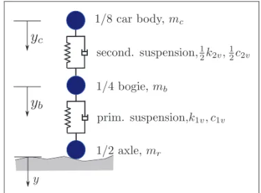
In the 2D analysis, the vehicle is modelled as a 1/8 railway car (see Figure 1). This model has two vertical degrees of freedom (DOF), in which there are two sprung masses: a mass of 1/8 car body mc and a mass of 1/4 bogiemb. The spring and damper elements represent the secondary and primary suspension con-necting the car body with the bogie and the bogie with the wheelset, respectively. The wheel is modelled as a mass of 1/2 wheelset mr, which has contact with the rail. This contact is modelled as a Hertzian spring (details for contact are included in the section on the wheel–rail contact element).
The equations of motion of the 1/8 vehicle model are written as
mcy€cþ
1
2c2vðy_cy_bÞ þ 1
2k2vðycybÞ ¼0 mby€bþc1vðy_by_rÞ þk1vðybyrÞ
1
2c2vðy_cy_bÞ 1
2k2vðycybÞ ¼0
8 > > > > < > > > > : ð1Þ
wherek2v,c2v,k1v,c1vare stiffness and damping coef-ficients of secondary and primary suspension along the Y axis. All parameters used in the simulation can be seen in Appendix 1. Table 1 shows the basic frequencies of vibration of this 2D vehicle model. This characterization considers the wheelset as fixed, i.e. the stiffness of the Hertzian spring for wheel–rail con-tact is not included.
3D model
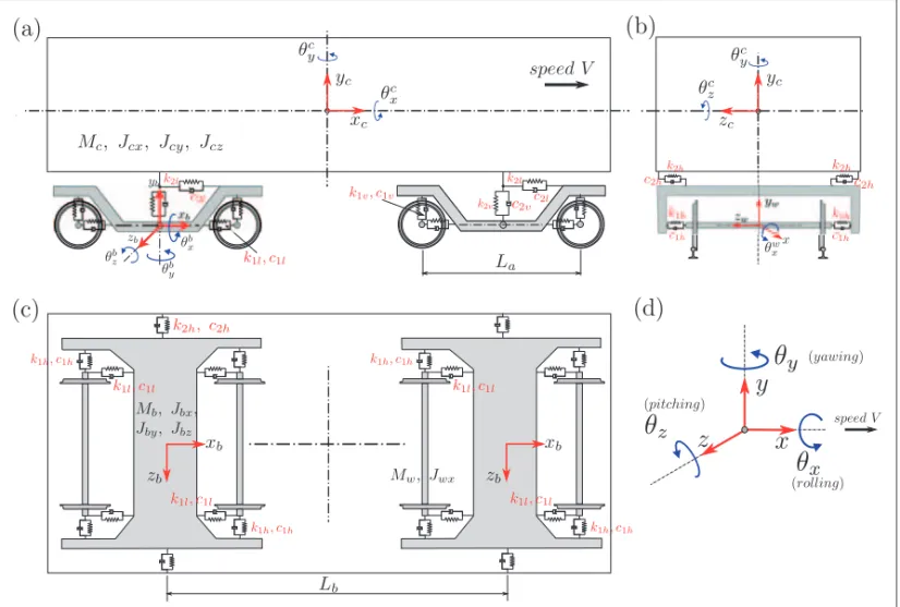
In the 3D analysis, some motions as rolling and lateral displacement of vehicle body can be produced by con-sidering the cross-level profiles, which only can be reproduced with a complete 3D vehicle model. Therefore, a complete 3D vehicle model is used in this study for giving more accurate analysis results than using the 2D vehicle model. The vehicle is mod-elled as a multibody system composed of individual rigid bodies with the mechanical properties corres-ponding to the high-speed vehicle that are listed in Appendix 1. In order to simplify the analysis, but with enough accuracy, the following assumptions are adopted.
1. The car body, bogies and wheelsets are considered as rigid bodies with associated mass and rotational inertia for each direction (see Figure 2).
2. The car body and the two bogies are connected by the secondary suspension, which is modelled by three linear spring–dashpot elements in the Y axis (k2v,c2v),Zaxis (k2h,c2h) andXaxis (k2l,c2l).
3. The bogies and wheelsets are connected by the primary suspension, which is represented by three linear spring–dashpot elements. The stiffness and damping coefficients are denoted ask1v,c1vfor theYaxis,k1h,c1hfor theZaxis andk1l,c1lfor the Xaxis.
Figure 1. A 1/8 vehicle model.
Table 1. Frequencies of vibration of the 2D vehicle model.
Vibration modes
No. of
mode Frequency (Hz) Description
4. The pitching and yawing motion of the wheelsets are not considered for the purposes of this study. 5. The wheels and rails always keep in contact.
With these assumptions, the car body is described by five DOFs:yc, zc, xc, cy, cz, with associated mass
Mc and mass moments of inertia Jcx, Jcy, Jcz. The bogie also has five DOFs:yb, zb, xb, yb, bz, and the
corresponding mass and mass moments of inertia are: Mb, Jbx, Jby, Jbz. For each wheelset, there are three DOFs:yw, zw, wx, the massMwand mass moment of inertiaJwx. In total, the vehicle model has 27 DOFs. The vehicle is developed and modelled as a rigid multibody system within the finite-element software ABAQUS. Indeed, the ABAQUS code will solve the full equations, which generate nonlinear and quad-ratic terms that originate naturally from rigid body dynamics in multibody simulations.20 Considering our study, which is limited to vertical dynamics, these nonlinear effects are not significant and can be neglected. Therefore, the equations of motion of the vehicle model can be linearized and written in a gen-eral form as
Mvu€vþCvu_vþKvuv¼Fv ð2Þ
where Mv, Cv, Kv are the total mass, damping and stiffness matrices. uv is the displacement vector and
Fv is the force vector applied on the vehicle.
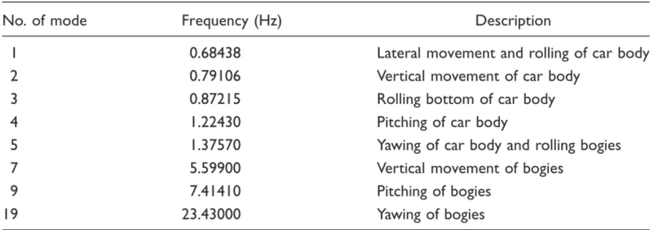
Some basic frequencies of the 3D model are listed in Table 2 without considering the stiffness of the Hertzian spring for wheel–rail contact (see the section on the wheel–rail contact element). It can be noted that the frequencies of vertical vibration in both the 2D and 3D model are very similar, comparing modes 2 and 7 in Table 2 with those in Table 1.
Modelling of the track
2D model
For modelling the two-dimensional track, several models have been reported in the literature.6–10,21,22 In general, the rail is modelled as a long beam (Euler or Timoshenko beam formulation) supported on a discrete model of the elastic foundation consist-ing of railpads, sleepers, ballast, subballast and subgrade.
The track model is discretized with finite elements (see Figure 3). An important feature of this model is that it must have enough length to capture all dynamic effects produced during the vehicle–track interaction. A track length of 90 m has been found sufficient and employed for this study. The rail has been simulated as a continuous Timoshenko beam including shear deformation, supported by pads, which are spring and damper elements. The sleepers are regarded as a concentrated mass. The ballast is
represented in a simplified manner by discrete spring and damper elements. The subballast is not con-sidered in this work. The subgrade is modelled as a viscoelastic element without mass. The values of rail-pad stiffness and ballast stiffness are taken from the data of the AVE Zaragoza track.23In order to calcu-late the ballast vibrating mass and the subgrade stiff-ness, the process proposed by Zhai et al.24 has been applied, in which the ballast vibrating mass is evalu-ated as
mba ¼b½lbhbðleþhbtgbÞ þleðh2bh
2 0Þtgb
þ4 3ðh
3
bh
3 0Þtg
2
b ð3Þ
The subgrade stiffness is calculated by
kc¼lsðleþ2hbtgbÞEf ð4Þ
wherebis the ballast density,hbis the depth of bal-last, le is the effective supporting length of the half
sleeper,lbis the sleeper width underside,bis the bal-last stress distribution angle,Efis the elastic modulus of the subgrade and h0¼hb(lslb)/(2tgb) is the height of the overlapping regions.
To determine the damping coefficient of the ballast and the subgrade, the damping coefficients of the bal-last and subgrade are assumed as 10% of their critical damping coefficientccrfor independent one DOF sys-tems. With this assumption, the damping coefficients of the ballast and subgrade can be determined by equation (5). All parameters of track used in this study can be seen in Appendix 1.
cb¼0:12
ffiffiffiffiffiffiffiffiffiffi
kbmt
p
, cc¼0:12
ffiffiffiffiffiffiffiffiffiffiffiffi
kcmba
p
ð5Þ
3D model
A 3D finite-element model of the ballast track struc-ture is also considered. The track has the same com-ponents and length as the 2D model. The rail is
Figure 3. The 2D dynamic model of the vehicle–track system.
Table 2. Frequencies of vibration of the 3D vehicle model developed in ABAQUS.
Vibration modes
No. of mode Frequency (Hz) Description
1 0.68438 Lateral movement and rolling of car body
2 0.79106 Vertical movement of car body
3 0.87215 Rolling bottom of car body
4 1.22430 Pitching of car body
5 1.37570 Yawing of car body and rolling bogies
7 5.59900 Vertical movement of bogies
9 7.41410 Pitching of bogies
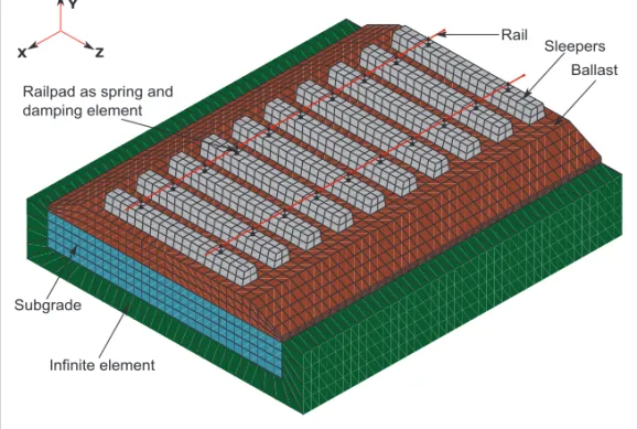
modelled as a 3D Timoshenko beam element, resting on discrete supports of railpads. The railpads are modelled as spring and damper elements, which have a vertical stiffness kp and viscous damping cp. The sleepers and ballast are modelled as 3D solid elements with the corresponding elastic properties (see Appendix 1). A perfect contact between the slee-pers and ballast layer is considered along the track length. Modelling the subgrade is an important issue, as, in principle, a detailed 3D model with stand-ard finite elements should extend to infinity in order to avoid reflection of stress waves transmitted from the structure. Of course, practical considerations make this unfeasible due to excessive computational cost. Among several authors who have studied this prob-lem, Costa25performed a comprehensive analysis and concluded that the use of infinite elements was the most precise and effective method. Hence, the infinite elements for the non-reflecting boundaries are used, as implemented in ABAQUS20 (see Figure 4). These elements are characterized by the fact that an expo-nentially decay term is multiplied by the shape func-tions associated with the direction extending to infinity to represent the amplitude attenuation effect of travelling waves. As a result, these elements absorb the energy of waves transmitted from the super-structure of the track, so that no reflections will occur at the boundaries.
The elastic modulus of ballast Eb is adjusted to have the same value of ballast stiffness used in the 2D model. Based on the value of ballast stiffness proposed in the 2D model (kb), from Zhai et al.24 the following expression for the elastic modulus of ballast may be obtained
Eb¼
a1þa2
a1a2
kb ð6Þ
where a1¼2(lelb)tgb/ln[(lels)/(lb(leþlslb))] and a2¼ls(lslbþ2leþ2hbtgb)tgb/(lblsþ2hbtgb).
The damping of ballast and subgrade are specified as part of a material definition. For this, ABAQUS provides use of Rayleigh damping.20To define this, it is necessary to specify two coefficients: for mass proportional damping andfor stiffness proportional damping. For each material, ballast and subgrade, the Rayleigh damping factors are determined by26
¼ 2!1!2
!1þ!2
, ¼ 2
!1þ!2
ð7Þ
The damping ratiox is determined as 10% in a fre-quency range [!1, !2]. For this study, the frequency
range [125, 1885] (rad/s) has been employed, in which the properties of the ballast and subgrade have strong effects on the track dynamics. Accordingly, the value of the Rayleigh damping factors used are:¼23.445 and ¼9.95021005. The test of decay of motion was taken to verify the correct values of and . The mechanical properties of the materials are listed in Appendix 1, and are consistent with the 2D model.
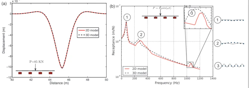
Figure 5 shows the static and dynamic character-ization of the track for both the 2D and 3D model. In the static response, a load of 85 kN at the centre point of the rail between two sleepers has been applied for both models. The static track response is very close for both models (see Figure 5a). For obtaining the dynamic track response, a harmonic load is applied at the centre point between two sleepers of the rail, and the amplitudes of displacement and force at the same point are obtained to define the track receptance. For both models, the ballast track has three peaks defining resonances, which
correspond to three fundamental vibration modes (see Figure 5b). The first resonance is due to the vibra-tion of rail-sleepers over the ballast layer (74 Hz for both models). The second peak occurs at 290 Hz for the 2D model and 273 Hz for the 3D model, and is due to the vibration of the rail over the sleepers. And the third peak corresponds to the pin–pin mode, asso-ciated with the bending of the rail between the sleeper supports (1065 Hz for the 2D model and 1050 Hz for the 3D model). It can be observed that there is a small difference in amplitude and frequency of the second and third peak between the 2D model and 3D model. The second and third vertical track resonant fre-quency is clear function of the characteristics of the rail and pads, but also depends on the damping prop-erties, masses of track structure components, etc. In both models, the rail and pads are modelled in the same way, but the other track components of sleepers, ballast and subgrade layer are not. This causes the damping properties and the masses of the track structure components to be not practic-ally the same in both models, which can produce a change in amplitude and frequency of these peaks.27 In general, the dynamic behaviour of the two models is similar.
Vehicle–track interactions
Generation of track irregularities
Coupling the vehicle system and railway track is realized through interaction forces between the wheels and the rail, where vertical track irregular-ity profiles (with wavelengths in the range [3–25 m]) is taken into account. The irregularity is generated from the power spectral density (PSD) of the verti-cal profile and cross level (see Clauss and Schiehlen28) according to the maximum considered limit (intervention limit) defined in EN13848-5:2008.29 The PSD functions used in this study are
defined by
VðOÞ ¼A O
2
c
ðO2rþO2ÞðO2cþO2Þ ð8Þ
CðOÞ ¼A l2
O2cO2
ðO2rþO2ÞðO2cþO2ÞðO2sþO2Þl ð9Þ
whereV(O) is the PSD of the vertical profile,C(O) is the PSD of the cross level andOis the spatial fre-quency (rad/m). The values of the constant factorsOr, Oc,Os,landAare
Or¼0:0206 rad=m ð10Þ
Oc¼0:8246 rad=m ð11Þ
Os¼0:4380 rad=m ð12Þ
l¼0:75 m ð13Þ
A¼3:65106ðrad mÞ ð14Þ
For the dynamic analyses, in order to achieve some statistical significance, the three different irregularity profiles have been generated with such limits consider-ing N¼901 discrete frequencies. The obtained data are used as input for the the vehicle–track interaction (see Figure 6).
In order to verify the correct generation of track irregularities, the conformity of such profiles is assessed, obtaining the PSD as the Fourier transform of the autocorrelation function of track irregularities generated. Comparisons of the PSD of the generated irregularities profiles and the analytical ones ((8 and 9)) are shown in Figure 7.
Wheel–rail contact elements
During the vehicle/track interaction, the forces are transmitted by means of the wheel–rail contact area.
On account of the geometry of the contact area between the round wheel and the rail, and under the assumptions that the wheel and rail are the same material with the elastic modulus E and Poisson’s ratio , using Hertz’s normal elastic contact theory,30the relationship between the vertical contact force Fv and the vertical relative deformation v is nonlinear and is given by
Fv¼ 3v=2CH, where,CH¼3ð12E2ÞðrrrwÞ1=4 ð15Þ
withrwthe wheel rolling radius andrrthe head radius of the rail cross section. A realistic common case of
rail type UIC60 with E¼2.11011N/m2, ¼0.3, rr¼0.3 m and rw¼0.455 m is considered in this study, for which the value of the Hertz coefficient CH is 9.3511010N/m3/2.
The wheel–rail contact is modelled as a Hertzian spring with one node at the centre of the wheel and the other node on the rail, as illustrated in Figure 8. In the literature, the Hertzian spring is often linear-ized by considering the relationship between the force and the displacement increments from the static wheel load. This assumption is valid when the vertical dynamic contact force does not exceed significantly the vertical static contact force or, in other words,
Figure 6. Generation of vertical irregularity profiles: (a) Vertical profiles; (b) Cross levels; (c) Vertical track irregularities.
the vertical relative deformation is not excessive. However, when the rail irregularities exist, the magni-tude of the vertical dynamic contact force may be much greater than the static one, and using the line-arized Hertzian spring does not lead to the real behav-iour of the Hertz contact mechanism. Therefore, in this study the nonlinear behaviour according to equa-tion (15) has been used for the contact.
Simulation results
In order to investigate and compare the 2D and 3D models, some simulations are performed with the models described above, using the finite-element pro-gram ABAQUS.20 For a consistent comparison between the results of the 2D model and 3D model, the uncoupled vehicle composed of four 1/8 vehicle models is used in the 2D simulation (see Figure 3). The calculation is done in the time domain, using the Hilber-Hughes-Taylor (HHT) time integration method to solve the transient problem. In this work, the dynamic effects of high-speed traffic load on the ballasted track are evaluated in a frequency range 0– 500 Hz. Consequently, the time step must be small
enough to accurately integrate a motion with this fre-quency range. A constant time step is used and has the value t¼0.2103
s, which satisfies the stability criteria (t/Tn40.1) recommended by Chopra.26 The Lagrange multiplier method is used for the con-tact constraint enforcement between the bottom node of the Hertzian spring and the rail surface. The numerical simulations are performed with different speeds (from 200 km/h to 360 km/h) and for each irregularity profile proposed. The following results have been obtained and will be discussed below:
. vertical displacement and acceleration of the bogie; . contact force between the wheel and the rail; . force transmitted to the railpads;
. vertical acceleration of the rail;
. envelope of the dynamic amplification factor of the wheel–rail contact force as a function of speed; . envelope of the dynamic amplification factor of the
force transmitted to the railpads.
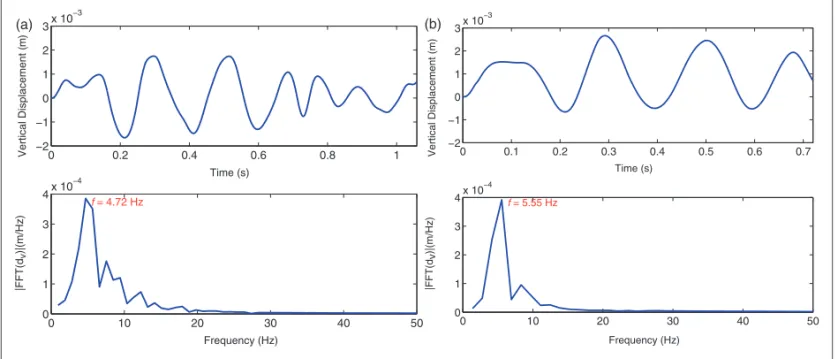
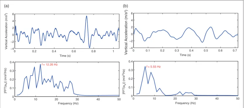
Figures 9 and 10 show the time history and fre-quency content (absolute value of the Fourier trans-form) of vertical displacement and acceleration of the bogie for both models when the train is moving at speed v¼300 km/h with track irregulari-ties. From Figure 9, it is noted that in both models, the dominant frequency of vibration is: f¼4.72 Hz for the 2D model and f¼5.55 Hz for the 3D model. These values are close to the fundamental frequency of vibration of the bogie of 5.6 Hz (Tables 1 and 2), and lie within the frequency of the irregularities, which have a range of [3.33–27.78] Hz for a speed v¼300 km/h. From Figure 10, it can be seen that for both models, the frequencies for the acceleration are in the low region (i.e. below 50 Hz); however, the acceleration results for the 2D model show a
Figure 9. Time history and frequency content of vertical displacement of bogie during the passage of the vehicle on track at speed v¼300 km/h with D11 profile: (a) 2D vehicle model result; (b) 3D vehicle model result.
significantly wider band of frequency content than for the 3D model.
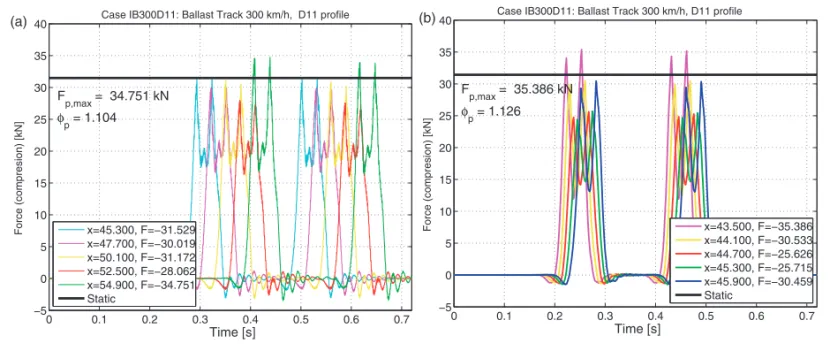
Figures 11 and 12 show the results of the contact force between wheel and rail at 340 km/h. Each figure consists of two subfigures, where (a) is the time his-tory and (b) is the frequency content of the dynamic component of contact force.
It can be observed that for both models, the fre-quency distributions of contact forces consist of a band in a low-frequency range (0–50 Hz) and some isolated resonant frequency peaks for higher frequen-cies. The lower frequency band is originated by the excitation frequency of the irregularities ([3.7831.48 Hz] for speed v¼340 km/h). The resonant peak at
approximately 157 Hz is due to the sleeper passage frequency (f¼v/d¼157.4 Hz for v¼340 km/h). This frequency has more influence in the 2D model than in the 3D model.
In Figure 13, a frequency content envelope map for different train speeds is gathered. It can be noted that both models show a frequency response band in the lower frequencies ([0–50] Hz) more or less con-stant for the entire speed range. This frequency band has higher amplitudes for the 3D model. Additionally, the peaks originated from the sleeper passage are produced at frequencies that increase linearly with speed, as expected. These peaks have greater amplitude for the 2D model. In spite of
Figure 10. Time history and frequency content of vertical acceleration of bogie during the passage of the vehicle on track at speed v¼300 km/h with D11 profile: (a) 2D vehicle model result; (b) 3D vehicle model result.
these differences, the qualitative behaviour of both models is similar.
Figure 14 shows the forces transmitted to some railpads during the passage of the vehicle travelling along the track at speedv¼300 km/h. The static force obtained in the railpad when the axle load (84.86 kN) is applied on the sleeper is used to compare with the dynamic results.
The vertical acceleration of the rail is represented in Figures 15 and 16 for different speeds of the vehicle. It is obvious that the magnitude of the acceleration of the rail is very sensitive to the vehicle speed: from 167 m/s2 forv¼200 km/h to 306 m/s2forv¼360 km/h in the 2D analysis, from 117 m/s2for v¼200 km/h to 314 m/s2 forv¼360 km/h. Comparing Figure 15a with Figure 15b, it can be concluded that in the frequency content, the results obtained in the 2D model and 3D model are
similar: both models have peaks at a similar frequency. Furthermore, it can be observed that in the range of frequencies studied ([0–500 Hz]), the lower frequencies has an important influence on the response of both models.
To interpret the results adequately and in dimen-sionless form, the dynamic impact due to the passing vehicle can be evaluated by using the concept of the dynamic amplification factor
’¼Fdyn
Fsta
ð16Þ
where Fsta is the static response and Fdyn is the maximum dynamic response obtained in the simula-tion. Figures 17 and 18 illustrate the dynamic amplification factors, respectively, for the wheel–rail
Figure 12. Contact force obtained in 3D model during the passage of vehicle with speedv¼340 km/h: (a) Time history; (b) Frequency content.
contact force and the forces transmitted to the rail-pads for each irregularity profile as a function of train speed, showing also an envelope for the different pro-files. It is noted that the irregularities of the track and the train speeds have a strong influence on the dynamic responses of railway track structures induced by traffic loads. In general, the amplification factor increases with speed. However, this is not always the case, and in some situations, critical velocities may be obtained.
Comparison between 2D and 3D results
Some representative results for both 2D and 3D simu-lations have been shown in Figures 11–18 in the pre-vious subsection on simulation results. The results of the 2D analysis are compared with the
corresponding 3D results, and the following general remarks are made.
. Differences between the dynamic response of the two models proposed are small. These differences are most apparent in the amplitude of response. In the frequency content of the contact force (see Figure 13), there is a difference in the frequency of the maximum amplitude: in the 2D model, the sleeper passage frequency has a notable influence, whereas in the 3D model, the frequency of the irre-gularities has more effects.
. The computational time consumed in the 2D model is relatively small (approximately 6 minutes per simulation), whereas the computational cost of the 3D simulation is very high (using a com-puter with six processors, the simulation time is 8
Figure 15. Time history and frequency content of vertical acceleration of the rail during the passage of vehicle on track at speed v¼200 km/h with D13 profile: (a) 2D model results; (b) 3D model results.
Figure 16. Time history and frequency content of vertical acceleration of the rail during the passage of vehicle on track at speed v¼360 km/h with D13 profile: (a) 2D model results; (b) 3D model results.
Figure 17. Envelope of dynamic amplification factor of wheel–rail contact force: (a) 2D model results; (b) 3D model results.
hours). Therefore, the 3D model is costly, not prac-tical from a computational point of view.
. The dynamic impact factor obtained with both analyses is very similar, demonstrating that the 2D model is capable of predicting the main features of the vertical dynamic response for both the vehi-cle and railway track components (see Figures 17 and 18).
Conclusions
. The dynamic effects of the high-speed traffic load on ballasted track have been studied using two inter-action models. The first one is the simplified 2D finite-element model, which neglects the lateral effects and considers a discrete model for ballast and subgrade. The second is a full 3D finite-element model with continuum elements for the ballast and subgrade and infinite elements in the boundary. . Several vertical track irregularity profiles are
generated from PSD and are included in the vehicle–track interaction. The nonlinear Hertz spring is considered for the wheel–rail contact, and the Lagrange multiplier method is used for the contact constraint enforcement. Analysing the results obtained in the interaction of both models, it is noted that the dynamic effects of high-speed traffic loads on the ballast tracks are sensitive both to the track irregularities and the vehicle speed.
. The dynamic response of the vehicle running on the track structure with irregularity profiles is predom-inantly due to the vibration of the bogie at a lower frequency than the fundamental frequencies of the track structure.
. Comparing the results of the 2D model with the 3D model, it has been found that although there is an unavoidable difference of the dynamic response between track models, there are similar levels of dynamic increments. Therefore, the 2D model can predict the vertical dynamic response with suffi-cient accuracy.
. On the basis of this study, it may be concluded that the 2D vehicle–track model can be employed for a quick and sufficiently accurate assessment of predicting the dynamic responses of the vehicle and the rail track components. The 2D model is also capable of examining the influence of the properties of the rail track and the vehicle components on the contact force and other dynamic responses of the rail track system.
Funding
This work was supported by the ‘Ministerio de Ciencia e Innovacio´n’ of the Spain Government through subpro-gram INNPACTO and project VIADINTEGRA [ref.
IPT-370000-2010-012]. The authors are also grateful for the sup-port provided by the Technical University of Madrid, Spain. K. Nguyen would like to express gratitude to AECID for a PhD grant during this study.
References
1. European Committee for Standardization, European Union.EN 1991–2:2003, Eurocode 1: actions on
struc-tures part 2: traffic loads on bridges. CEN, Brussels,
2003.
2. European Committee for Standardization, European Union. EN 1990:2002/A1:2005–Eurocode–basis of structural design. Annex A2. Application for bridges. CEN, Brussels, 2005.
3. European Railway Agency, European Union.Technical specification for interoperability relating to the infra-structure sub-system of the trans-European high-speed rail system. ERA, 2007.
4. Knothe K and Grassie SL. Modelling of railway track and vehicle/track interaction at high frequencies. Veh
Syst Dyn1993; 22(3-4): 209–262.
5. Dahlberg T. Vertical dynamic train/track interaction – verifying a theoretical model by full-scale experiments.
Veh Syst Dyn1995; 24(1): 45–57.
6. Cai Z and Raymond GP. Modelling the dynamic response of railway track to wheel/rail impact loading.
Struct Eng Mech1994; 2: 95–112.
7. Zhai W and Cai Z. Dynamic interaction between a lumped mass vehicle and a discretely supported continuous rail track. Comp Struct 1997; 63: 987–997.
8. Sun YQ and Dhanasekar M. A dyanmic model for the interaction of the rail track and wagon system. Int J
Solids Struct2002; 39: 1337–1359.
9. Esveld C. Modern railway track. MRT Productions
2001.
10. Lei X and Noda NA. Analyses of dynamic response of vehicle and track coupling system with random irregu-larity of track vertical profile. J Sound Vib2002; 258: 147–165.
11. Lou P and Zeng QY. Vertical vehicle track coupling element. Proc IMechE, Part F: J Rail and Rapid Transit2006; 220(3): 293–304.
12. Yang SC. Enhancement of the finite-element method for the analysis of vertical train-track interactions.
Proc IMechE, Part F: J Rail and Rapid Transit 2009;
223(6): 609–620.
13. Popp K, Kaiser I and Kruse H. System dynamics of railway vehicles and track. Archive Appl Mech 2003; 72: 949–961.
14. Sun YQ, Dhanasekar M and Roach D. A three dimensional model for the lateral and vertical dynamics of wagon track systems. Proc IMechE, Part F: J Rail
and Rapid Transit2003; 217(1): 31–45.
15. Kumaran G, Menon D and Nair KK. Dynamic studies of railways sleepers in a track structure system.J Sound Vib2003; 286: 485–501.
16. Lundqvist A and Dahlberg T. Load impact on railway track due to unsupported sleepers.Proc IMechE, Part
F: J Rail and Rapid Transit2005; 219: 67–77.
18. Zhai W, Wang K and Cai C. Fundamentals of vehicle track coupled dynamics. Veh Syst Dyn 2009; 47(11): 1349–1376.
19. Dahlberg T. Railway track stiffness variations conse-quences and countermeasures. Int J Civil Eng 2010; 8(1): 1–12.
20. Dassalt Systemes SIMUIA Corp. ABAQUS analysis
user’s manualv, 6.11. Dassalt Systemes SIMULIA
Corp., 2011.
21. Ishida M and Suzuki T. Effect on track settlement of interaction exited by leading and trialing axles.QR of RTRI2005; 46(1).
22. Knothe K and Wu Y. Receptance behaviour of railway track and subgrade. Archive Appl Mech 1998; 68: 457–470.
23. Melis M. Embankments and ballast in high speed rail. Fourth part: high-speed railway alignments in Spain. Certain alternatives. Revista Obras Pu´blicas 2007; 3476: 41–66.
24. Zhai WM, Wang KY and Lin JH. Modelling and experiment of railway ballast vibrations. J Sound Vib
2004; 270(4–5): 673–683.
25. Costa PMBA. Vibrac¸o˜es do sistema via-macic¸o induzidas por tra´fego ferrovia´rio. Modelac¸a˜o nume´rica
e validac¸a˜o experimental. Porto: Universidade do
Porto, 2011.
26. Chopra AK.Dynamics of structures: theory and appli-cations to earthquake engineering. 2nd ed. Prentice Hall, 2000.
27. Ma L, Liu W, Zhang H, et al. Influence of track par-ameters on rail frequency response function based on analytical solution. In:Advances in environmental vibra-tion – proceedings of the fifth internavibra-tional symposium on
environmental vibration. Science Press, 2011,
pp.700–706.
28. Clauss H and Schiehlen W. Modeling and simulation of railways bogie structural vibrations.Veh Syst Dyn1998; 29(1): 538–552.
29. European Committee for Standardization, European Union. EN 13848-5:2008 railway applications–track–
track geometry quality part5:geometric quality levels. CEN, Brussels, 2008.
30. Johnson KL. Contact mechanics. Cambridge: Cambridge University Press, 1985.
31. Ministerio de Fomento de Espan˜a. ‘‘Instruccio´n de acciones a considerar en el proyecto de puentes de fer-rocarril (IAPF)’’. Direccio´n General de Ferrocarriles, Madrid, 2007.
Appendix 1: Properties of models
Table 3. Main parameters of railway vehicle and track used in the simulation.
Notation Parameter Value
Vehicle system
Lb Distance between bogies (m) 17.375
La Distance between wheelsets in bogie (m) 2.5
Mc¼8mc Mass of car body (kg) 53,500
Jcx Mass moment of inertia of car body aboutXaxis (kg m2) 9.57104
Jcy Mass moment of inertia of car body aboutYaxis (kg m2) 1.69106
Jcz Mass moment of inertia of car body aboutZaxis (kg m 2
) 1.69106
Mb¼4mb Mass of bogie (kg) 3500
Jbx Mass moment of inertia of bogie aboutXaxis (kg m 2
) 2231
Jby Mass moment of inertia of bogie aboutYaxis (kg m2) 4569
Jbz Mass moment of inertia of bogie aboutZaxis (kg m2) 2802
Mw¼2mr Mass of wheelset (kg) 1800
Jwx Mass moment of inertia of wheelset aboutXaxis (kg m2) 880
k2v Stiffness coefficient of secondary suspension alongYaxis (kN/m) 410
c2v Damping coefficient of secondary suspension alongYaxis (kN s/m) 45
k2h Stiffness coefficient of secondary suspension alongZaxis (kN(m) 315.6
c2h Damping coefficient of secondary suspension alongZaxis (kN s/m) 50
k2l Stiffness coefficient of secondary suspension alongXaxis (kN(m) 500
c2l Damping coefficient of secondary suspension alongXaxis (kN s/m) 65.4
k1v Stiffness coefficient of primary suspension alongYaxis (kN/m) 873
c1v Damping coefficient of primary suspension alongYaxis (kN s/m) 24
k1h Stiffness coefficient of primary suspension alongZaxis (kN/m) 5100
c1h Damping coefficient of primary suspension alongZaxis (kN s/m) 58.86
k1l Stiffness coefficient of primary suspension alongXaxis (kN/m) 24,000
c1l Damping coefficient of primary suspension alongXaxis (kN s/m) 19.62
Table 3. Continued
Notation Parameter Value
Track system
L Model length (m) 90.0
hb Ballast thickness (m) 0.40
ls Sleeper spacinga(m) 0.60
Rail UIC60
kp Railpad stiffnessb(MN/m) 100
cp Railpad damping
a
(MN s/m) 0.015
kb Ballast stiffnessb(MN/m) 100
cb Ballast dampingc(MN s/m) 0.0253
kc Subgrade stiffness (MN/m) 80
cc Subgrade dampingc(MN s/m) 0.0455
mt Half sleeper mass
a
(kg) 160
mba Ballast mass (kg) 646
Eb Elastic modulus of ballast (MN/m2) 68.44
Ef Elastic modulus of subgrade (MN/m2) 90
Es Elastic modulus of sleeperc(MN/m2) 38.45103
b Ballast densitya(kg/m3) 1800
f Subgrade densitya(kg/m3) 1800
s Sleeper density
a
(kg/m3) 2400
lb Sleeper width undersidea(m) 0.3
le Effective supporting length of half sleepera(m) 0.95
b Ballast stress distribution anglea 35
*
a
Assumed value.15,18,24,31
b
The values taken from the data of AVE Zaragoza track.
c