Models for Lateral Dynamic Interaction of High-Speed Trains and Bridges
P. Antol´ın1, J. Oliva1, J. M. Goicolea1, M. ´A. Astiz1
1Department of Mechanics and Structures, School of Civil Engineering, Technical University of Madrid, Profesor Aranguren s/n 28040, Madrid, Spain
email: pablo.antolin, javier.oliva, jose.goicolea, miguel.a.astiz, @upm.es
ABSTRACT: In this work a methodology for analysing the lateral coupled behavior of large viaducts and high-speed trains is proposed. The finite element method is used for the structure, multibody techniques are applied for vehicles and the interaction between them is established introducing wheel-rail nonlinear contact forces. This methodology is applied for the analysis of the railway viaduct of the R´ıo Barbanti˜no, which is a very long and tall bridge in the north-west spanish high-speed line.
KEY WORDS: Train-Bridge Interaction; Dynamics; High-Speed Railway; Nonlinear wheel-rail contact
1 INTRODUCTION
In Spain, new railway lines are currently under construction in regions with very deep valleys. For that reason, strong winds appear over vehicles and structures and very tall and long viaducts are being built. Sometimes, due to that, these bridges have a very low lateral stiffness and lateral dynamic effects, that may endanger safety of circulation, could appear. In this work a realistic vehicle-bridge interaction model is proposed which considers lateral effects for studying this kind of cases.
As it is described in [1], the vehicle-bridge interaction systems are composed of five main issues: structure and vehicle modelling, track irregularities, wheel-rail contact and numerical solution algorithm for equations.
With regard to structure, the finite element method is widely used in this kind of analysis. Most of the authors use beam and truss elements, as it can be seen in [1], [2], [3], [4], [5], [6], [7] and in this work. However, other type of elements, such as shell [8] or solid [9], are applied too.
Multibody dynamic models, which are composed of rigid bogies, springs, dampers and constraints, are used for the vehicles. For vehicle-structure interaction analysis linearized models are applied, as it can be found in [1], [2], [3], [4], [5], [6], [7], [10], [11] and [12]. More realisitic models, which consider nonlinear effects, are described in [13] and [14].
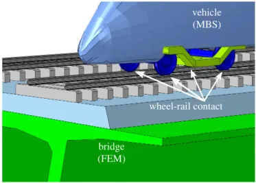
The key point of the vehicle-bridge interaction is to establish the geometric and dynamic relationships between both subsystems (see Figure 1). For establishing these relationships wheel-rail contact theories are used. With regard to the geometric relationship in the wheel-rail contact it is very common to consider that wheels have the same state of motion with their relative points on the rail and it can be seen in [1], [4], [5], [8], [10], [11], [15], [16] and [17]. Furthermore, in order to take into account the hunting movement of the train wheelsets, in some works this movement is imposed as a sinusoidal relative desplacement between the wheelset and the track, as it is developed in [1], [4], [5], [11] and [17]. In other way, other models consider free relative displacements between wheels and rails. In these cases it is necessary to introduce
the normal and tangential forces which appear in the contact between wheels and rails. In normal contact, the nonlinear Hertz theory [18] it is very common and it is used in this work and in [2], [7], [13] and [14], but in other way, a linearization of this theory can be applied as in [6]. For tangential contact the Kalker Linear Theory [19] is widely applied in vehicle-bridge interaction system as it occurs in [2], [3], [6] and [7]. However, in other works [13], [14], which are focused only on vehicles, more realistic tangential models are applied. Kalker USETAB table [20], which is based on Kalker Variational Theory [21], is very common in train dynamic analysis and it is used here.
In addition, it is necessary to introduce track irregularities in the geometric relationships between the wheelset and the track. Irregularity profiles can be generated using power spectral density functions as it is explained in [22] and applied on [6], [7] and in this article. In other way, irregularity profiles can be measured directly on the track, as in [1], [3] and [4], and then introduced in the numerical model.
vehicle (MBS)
wheel-rail contact
bridge (FEM)
For solving the dynamic system, both subsystems can be integrated separately and an iteration is established in each time time for achieving forces and displacements compatibility between them. This method is applied in [1], [6], [7], [11] and [23]. In other way, a single set composed of coupled equations of both subsystems can be solved directly, as in this work and in [3], [4], [5], [10] and [16].
To use finite elements, multibody dynamic techniques and an interaction between them based on contact forces provides a very flexible and powerful method for analyze any kind of structures and vehicles. Thus, any kind of nonlinearities (material, geometric, etc.) and constraints could be introduced in the formulation using this method.
2 NUMERICAL MODEL
The vehicle-bridge interaction system is composed of the vehicle and bridge subsystems and the interaction relationships between them. Thus, in this Section the equations that govern all of these parts are presented. Cartesian coordinate axes are used in both subsystems: xis along bridge lontigudinal direction, z
points upward andyis defined according to the right-hand rule. In addition, θx, θy andθz correspond to rotations around the coordinate axes (see Figure 2).
z
x θy
H
T2 T1
W4
2d1 2d2 2d1
x y θz
r0
h3
h2
h1
W3 W2 W1
Figure 2. Vehicle schema.
2.1 Vehicle model
For modelling the vehicle behaviour, the multibody dynamics method is applied. Thus, car body, bogies and wheelset are considered rigid bodies, and the primary and secondary suspension are defined using linear springs and dampers. For the vehicle model, the following assumptions are considered: (A1) Small displacements are assumed and nonlinear geometric effects are neglected.
(A2) The train is supposed to cross the bridge at a constant speedvand the path of the track to be straight.
(A3) The train is composed of independent cars: neither bogies nor wheelsets are shared by two different cars.
(A4) A constant velocity valong x axis is considered for all the bodies of each car, therefore the degrees of freedom of car-bodies and bogies arey,z,θx,θy andθz. For wheelset, θy is assumed to be constant because ˙θy=v/r0, beingr0the nominal rolling radius of wheels.
Using the multibody dynamics method for small displacements, the equations of motion of the vehicle can be written as:
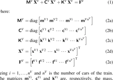
MVX¨V+CVX˙V+KVXV=FV (1)
where:
MV=diaghmV1mV2··· mVi ··· mV nVi (2a)
CV=diaghcV1cV2 ···cVi ···cV nVi (2b)
KV=diaghkV1kV2···kVi ··· kV nVi (2c)
XV=hxV1xV2 ···xVi ···xV nViT
(2d)
FV=hfV1fV2 ···fVi ···fV nViT
(2e)
being i=1, . . . ,nV andnV is the number of cars of the train.
The matrices mVi, cVi and kVi are, respectively, the mass, damping and stiffness local matrices of the vehiclei. A detailed description of the terms of these matrices can be found in [3].fVi
is the local forces vector of the cari. In this article, only gravity loads are applied on the vehicle.
The degrees of freedom of one car can be expressed as a function of the degrees of freedom of each body in the car:
xVi=xVi
H xViT1xViT2xViW1xViW2xViW3xViW4T, (3) where H, T and W correspond to car body, bogies and wheelsets, respectively (see Figure 2) and their degrees of freedom are:
xVi
H =yViH zViH θxVi,H θyVi,HθzVi,HT (4a) xVi
T j=yViT jzViT jθxVi,T jθyVi,T jθzVi,T jT j=1,2 (4b) xVi
W j=yViW jzViW jθxVi,W jθzVi,W jT j=1, . . . ,4 (4c) 2.2 Bridge model
For modelling the bridge, the finite element method has been applied and beam elements have been used. The assumptions that have been made are:
(A5) Only small displacements and linear elastic materials are considered.
(A6) The rails are supossed to be ridigly attached to the deck section.
(A7) Elastic effects on rails are neglected.
Thus the equations that govern the behaviour of the structure are written as:
MBX¨B+CBX˙B+KBXB=FB (5)
It is assumed thatFB=0because no external loads are applied
y z θx
ey ez
T
D
Figure 3. Bridge deck.
coordinatex, the gravity centreDand trackTdisplacements are defined as (see Figure 3):
xB
D(x) =yBD(x)zBD(x)θxB,D(x)θzB,D(x)T , (6a) xB
T(x) =yBT(x)zBT(x)θxB,T(x)θzB,T(x)T. (6b)
The displacement of the centroid of deck beam sectionDcan be obtained as a function of nodal displacements:
xB
D(x) =TBD(x)XB, (7)
beingTBD(x):
TBD(x) = 0 ···0 TBD,m(x)TBD,m+1(x)0 ···0 (8)
andXB:
XB= xB
1 ··· xBm−1xBmxBm+1xBm+2···xBnB
T
, (9)
wheremandm+1 are the nodes of the element in which the wheelset is over (Figure 4). The nodal degrees of freedom of the nodemof the structure are:
xB
m=xBmyBmzBmθxB,mθyB,mθzB,mT. (10)
i,j
Nodem Nodem+1
Elementk xB
m+1
xB m+1
x
Figure 4. Wheelset between two nodes of the bridge deck.
The interpolation matrixTBD,m(x)is defined as:
TBD,m+k=
0 N1+k 0 0 0 Nˆ1+k
0 0 N1+k 0 −Nˆ1+k 0
0 0 0 N3+k 0 0
0 N0
1+k 0 0 0 Nˆ10+k
(11)
Euler-Bernoulli beam elements were used, thus, shape functions are third order Hermite polynomials (N) for bending defor-mation interpolacion and linear functions ( ˆN) for axial and torsional, being k=0,1 and (•)0= dd(•x). Thus, taking into
account verticalezand lateraleytrack eccentricity and the track irregularities, displacements of pointBcan be defined as:
xB
T(x) =TBTTBD(x)xB+Γ(x), (12)
whereΓΓΓ(x)is the track irregularities profile vector [24]:
ΓΓΓ(x) = [Γy(x)Γz(x)Γθx(x)0]T (13)
whose components are: Γy(x) the lateral aligment irregularity profile,Γz(x)the vertical surface irregularity profile andΓθx(x)
and the rotation corresponding to cross level irregularity profile.
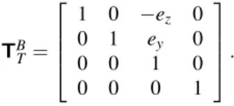
TBT is the transformation matrix:
TBT=
1 0 −ez 0
0 1 ey 0
0 0 1 0
0 0 0 1
. (14)
Neglecting the first and second time derivatives ofTBT(x), the
velocity and acceleration ofT are:
˙
xB
T(x) =TBTTBD(x)x˙B+d ΓΓΓ(x)
dx v, (15a)
¨
xB
T(x) =TBTTBD(x)x¨B+d
2ΓΓΓ(x)
dx2 v2. (15b)
2.3 Vehicle-bridge interaction
For establishing the interaction between the vehicle and the structure the contact interaction forces between them are introduced into the equations. In this way, a coupled system of equations considering the vehicle (1) and bridge (5) equations and the contact interaction forces is written:
MV 0 0 MB
¨
X+
CV 0 0 CB
˙
X
+
KV 0 0 KB
X=
FV
+FVc FB+FB c
,
(16)
where FV
c is the vector of forces applied on the vehicle as a
consequence of the interaction with the structure, and FB c, on
the structure.Xis:
X=
XV XB
. (17)
FV
c andFBc depend on the vehicle and bridge displacements and
velocities and time.FV
c is defined as:
FV c =
h
fV1
c fVc2···fVic ···fV n V c
i
, (18)
where the interaction forces vector of each vehicle is:
fVi c =
h
0 0 0fVc,1W1fVc,1W2fcV,1W3fVc,1W4i. (19)
fVi
c,W j is the contact forces vector that appear in wheelset j of
vehicleias a consequence of interaction with the bridge. The superscriptViand subscriptW j, which refer to the wheelset j
of the vehiclei, are supressed in the rest of the article.
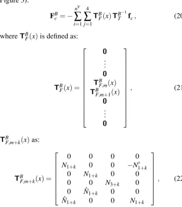
applied on the bridge deck are obtained as a function offc(see
Figure 3):
FB c=−
nV
∑
i=1 4
∑
j=1
TBF(x)TBT−1fc, (20)
whereTBF(x)is defined as:
TBF(x) =
0
...
0 TBF,m(x) TBF,m+1(x)
0
...
0
, (21)
TBF,m+k(x)as:
TBF,m+k(x) =
0 0 0 0
N1+k 0 0 −N10+k
0 N1+k 0 0
0 0 N3+k 0
0 Nˆ1+k 0 0
ˆ
N1+k 0 0 N1+k
, (22)
k=0,1, and x is the longitudinal position of the wheelset
considered.
The equation (16) is solved using the HHT Method [25], which is a implicit time integrator. Due to that, tangent matrices are needed for solving the system. Thus, the tangent matrices of contact forces are computed:
Kc=dFc
dX , (23a)
Cc=dFc
d ˙X , (23b)
where:
Fc=
FV
c FB c
. (24)
The expressions of the tangential forces applied in this work have not an analytical time derivative, and due to that, tangent matrices have to be calculated using numerical jacobians.
2.4 Nonlinear contact forces
The wheel-rail contact forces are developed in this Section. Considering some assumptions, that are expossed below, this problem can be split in three main parts:
Geometric problem: it consists on computing the main geo-metric variables which depend on the relative displacements between wheel and rail.
Normal problem: considering the geometric variables obtained before, the contact ellipse dimensions and the normal stress distribution is calculated using the Hertz theory [18].
Tangential problem: the tangential forces, which depend on the contact geometry, normal stresses and relative velocities between wheel and rail, are computed.
According to [21], if the wheel and rail materials have the same mechanical properties, the three problems can be studied separately: geometric problem is solved firstly, normal problem secondly and tangential problem thirdly.
2.4.1 Geometric contact problem
For obtaining the main geometric variables of the contact problems serveral assumptions are made:
(A8) Separations between wheel and rail are not allowed. (A9) The wheel-rail contact appears only in one area.
(A10) Only rigid body movements perpendicular toxaxis are considered for the wheelset and the track.
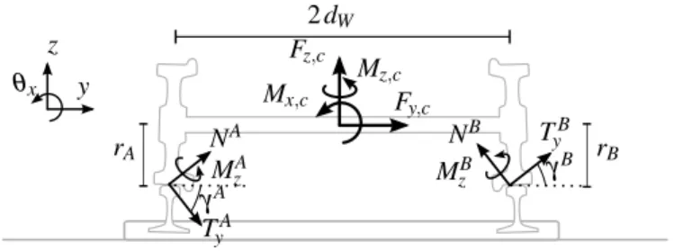
Considering that the distance between two wheelset of the same wheelset is 2dW, the geometric variables can be computed as a function of only variable: the lateral displacement of the wheelset relative to the track∆yW. These geometric variables for wheelsAandB(Figure 6) are (see Figure 5):
• rAandrB: the rolling radii of both wheels at the contact point. • γAandγB: the angle between horizontal and contact plane (the
plane where the contact ellipse is contained).
• kaA,kbA,kaBandkbB: ellipse dimension coefficients that depend
on the curvatures of wheel and rail in the two main directions at the contact point (see [18]). ais the ellipse semiaxis alongxc, andbalongyc.
• ∆zWˆ and∆θxˆ,W: relative vertical displacement and rotation
between the wheelset and the track, considering only geometric conditions.
zc γ
xc
yc
rr,y r
rw,y
Figure 5. Main variables of the contact geometry.
In this article, realistic wheel and rail profiles are considered (biconic profiles are avoided), due to that, when the relative lateral displacements of the wheelset respect to the track are small, the variation of the previous variables is linear. However, when the displacements become larger, contact between the flange of the wheel and the rail occurs, and the variation becomes nonlinear.
The relative displacements of the wheelset of vehicle respect to the track are:
∆yW =yW−yBT(x), (25a)
∆zW =zW−zBT(x), (25b)
being yW, zW, θx,W andθz,W the absolute displacements and
rotations of the wheelset.
2.4.2 Normal contact problem
The Hertz theory [18], for solving the shape and dimensions of the contact surface and the normal stress distribution, take into consideration the following assumptions:
(A11) At contact point, contact surfaces are continuous and nonconformal.
(A12) No plastic deformation is considered and strains are supposed to be small and elastic.
(A13) Stresses are neglected far from contact point.
(A14) Friction between surfaces does not affect to normal problem.
(A15) Quadratic functions of two variables can be used to define the wheel and rail surfaces near to contact point.
With these assumptions, contact area is considered an ellipse and normal stress distribution an ellipsoid.
The ellipse semiaxes can be computed as:
ak=kak(∆yW)
1
−ν
G Nk
1/3
(26a)
bk=kbk(∆yW)
1
−ν
G Nk
1/3
(26b)
wherek={A,B},Gis the shear stress modulus,ν the Poisson
coefficient of wheels and rails andNkthe contact normal force
in wheel-rail pair (it is explained below how to compute these normal forces). The coefficients ka
k andkbk, which depend on ∆yW, are computed before the calculation and depend on the main curvatures of wheel and rail at contact point (see [26]).
2.4.3 Tangential contact problem
In this problem the tangential contact forces are computed. They appear as a consequence of a rolling and sliding motion between wheels and rails. In each point of the contact surface the shear stress value can not be greater than the normal stress times friction coefficient. Thus, in the contact ellipse adhesion and slip areas could appear.
The main variables of the tangential contact are the creepages, which are defined as the non dimensional relative velocities between wheel and rail. ζk
x, ζyk and ζRk are, respectively,
longitudinal, lateral and rotational creepages of wheel-rail pair
kand can be expressed as:
ζk
x =1−rkr
0±
∆θz˙,W
v dW (27a)
ζk
y =1v ∆yW˙ +∆θx˙,Wrkcosγk
+ ∆zW˙ ±∆θx˙,WdWsinγk
(27b)
ζk
R=−sinrγk
0 (27c)
where the upper sign of ± and ∓ in the above equations corresponds to the wheel-rail pair A, and the lower, to B (see Figure 6).
Depending on the assumed hypothesis, different methods for solving tangential contact exist. The Kalker Variational
Method [21] is a very accurate method for computing tangential forces, however, due to it is computationally very expensive, it can not be applied in an analysis like that. The USETAB approximation [20], proposed by Kalker, is used in this work. This method obtains the tangential forces in a pre-calculated table whose input variables are the contact normal force, the ellipse semiaxes, the friction coefficient and the creepages, and the output variables are the tangential forces in longitudinal
Tk
x and lateral Tyk local directions and moment around normal
directionMk
z. The values of this table have been computed using
the Kalker Variational method for different values of the input variables.
2.4.4 Vehicle-structure interaction forces
As it has been seen above, vertical relative displacement ∆zW
and relative rotation ∆θx,W can be computed as geometric
variables, without regard to dynamic aspects. Thus, the relative displacements computed as geometric variables and those obtained from the dynamic response of vehicle and structure must be equal:
∆zW=∆zWˆ (∆yW), (28a)
∆θx,W=∆θˆx,W(∆yW). (28b)
For imposing these constraints, a penalty force and moment are introduced in wheelsets gravity centre:
Fz
c =kz(∆zWˆ (∆yW)−∆zW)3/2, (29a) Mx
c=kθ ∆θxˆ,W(∆yW)−∆θx,W3/2. (29b)
These nonlinear penalty expresions derive from the approach expression bewtween two bodies of the Hertz theory. Stiffness coefficientskz andkθ depend on∆yW andNWk, but in order to
simplify the equations, they are computed considering only the train own weight in a static case and∆yW=0.
2dW Fz,c
Mz,c Fy,c Mx,c
MA z
γA γ
B rB rA NA
TA y
NB TB y MB
z z
y θx
Figure 6. Wheelset equilibrium.
The forces applied on the wheelset gravity centre, shown in Figure 6, can be written as:
Fy
c =−NAsinγA+TyAcosγA−NBsinγB+TyBcosγB, (30a) Fcz=NAcosγA+TyAsinγA+NBcosγB+TyBsinγB, (30b) Mx
c= −NAcosγA−TyAsinγA+NBcosγB
+TyBsinγBdW+ TyAcosγA−NAsinγArA + −NBsinγB+TyBcosγBrB,
(30c)
Using equations (29), (30b) and (30c), normal forces NA and NB, which are needed to compute the tangential forces and
moments, can be obtained and applied to compute the values of Fcy andMcz. Thus, the equation set (30) is nonlinear and,
in order to solve a linear system, as it is proposed in [13], the normal forces computed in the previous time step are used for computing the tangential forces in the current time step. Before obtainingFcyandMcz, the contact forcesTyA,TxB,TyBand
momentsMA
z andMzBmust be computed using normal forces of
the previous time step and the creepages of current step.
3 RESULTS
3.1 General information
An application of the method presented above is shown in this Section. For this example, the Barbanti˜no bridge, in the northwest spanish high speed line (under construction), is studied when the vehicle Siemens ICE 3 crosses it.
The deck of Barbanti˜no bridge is a 1176 m length continuous beam and it is composed of 18 spans, as shown if Figure 7. The 1st and 18th span are 52 m length and the rest are 67 m length, and some of its piers are larger than 90 m. For that reason, the lateral frequencies of the bridge are very low (see Table 1). The first vibration mode can be seen in Figure 8. The deck section
Table 1. First natural frequencies of the Barbanti˜no bridge (values in Hz).
1st 2nd 3rd 4th
0.294 0.424 0.456 0.589
is a prestressed concrete girder whose width and depth are 14 m and 4.94 m, respectively, and its eccentricities, which appear in
(14), areey=2.50 m andez=2.05 m.
The Rayleigh damping method has been used for determining the damping matrix of the structure subsystem. The first two natural frequencies and 2% damping ratio have been used.
The train that has been used in the calculations is an approximation of the Siemens ICE 3 (real data is not known) composed of 8 cars (see Figure 9) whose length is 24.775 m. It
is a distributed power train, and, for that reason, all the cars
Figure 8. First vibration mode of Barbanti˜no bridge.
Figure 9. Siemens ICE 3 train.
ares supposed to have the same geometrical and mechanical properties.
Irregularity profiles have been generated using a power spectral density method defined in [22] and a 100 m sample can be seen in Figure 10.
0 20 40 60 80 100
−2
0 2
x[m] Γy
,
Γz
[mm]
Γy Γz
Figure 10. Sample of 100 m length of the lateral and vertical alignment irregularities used in the analysis.
In Section 3.2 the dynamic response of the structure and the vehicle, when the train crosses the bridge at different velocities, are shown.
3.2 Bridge and vehicle response
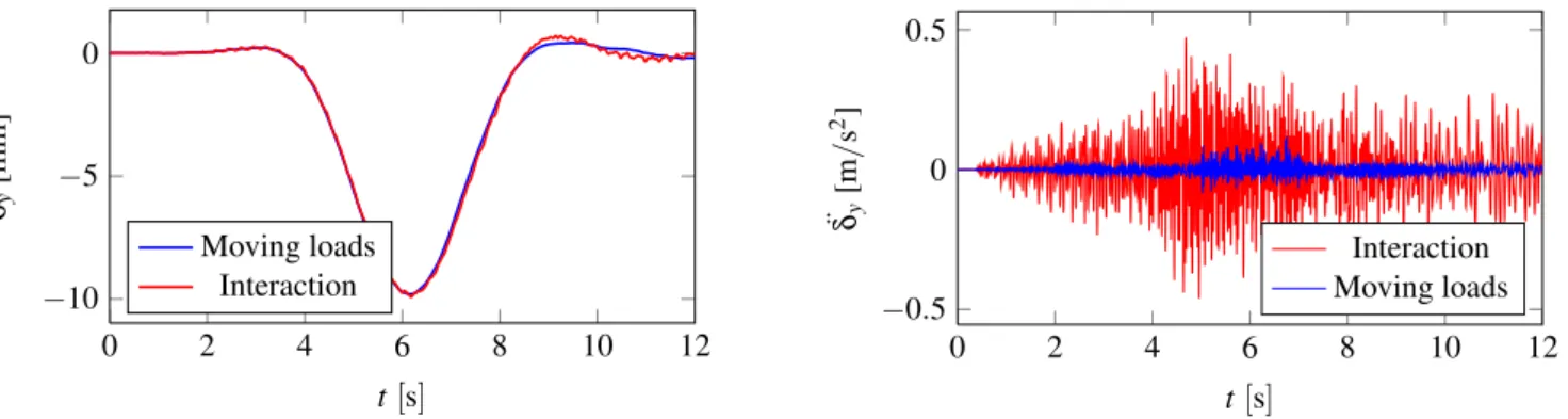
In Figures 11 and 12 lateral displacements of centre of the 8th span (near to the tallest pier) at pointT(see Figure 3) can be seen for train velocities 200 km/h and 350 km/h. In these figures the
results obtained with the method propossed above are compared with those obtained using the moving loads method (see [27]) which does not consider the interaction between vehicle and structure. As it is shown in these figures, the responses obtained with both methods are very similar. However, big differences can be appreciated in accelerations (Figures 13 and 14) due to the moving loads method does not take into consideration track irregularities which are an important source of excitation.
z
y x
L=1176 m 67 m
52 m
81
.
7
m
97
.
9
m
Figure 7. Global view of Barbanti˜no bridge.
0 5 10 15 20 25
−8
−6
−4
−2
0
t[s] δy
[mm]
Moving loads Interaction
Figure 11. Lateral displacements of the centre of the 8th span of the bridge for a train speedv=200 km/h.
0 2 4 6 8 10 12
−10
−5
0
t[s] δy
[mm]
Moving loads Interaction
Figure 12. Lateral displacements of the centre of the 8th span of the bridge for a train speedv=350 km/h.
The analysis presented in this article does not consider the wind action, but it is going to be introduced in future works and as a consequence, adding wind forces to the vehicle response, train safety may be endangered.
4 CONCLUSIONS
A realistic vehicle-bridge interaction method has been proposed. This method uses the linear beam elements for the structure and a linearized multibody model for the the vehicle. Furthermore, an interaction based on nonlinear wheel-rail contact forces is established between them. This methodology can be applied
0 5 10 15 20 25
−0.2 −0.1
0 0.1
t[s]
¨δ[my
/
s
2]
Interaction Moving loads
Figure 13. Lateral accelerations of the centre of the 8th span of the bridge for a train speedv=200 km/h.
0 2 4 6 8 10 12
−0.5 0 0.5
t[s]
¨δ[my
/
s
2]
Interaction Moving loads
Figure 14. Lateral accelerations of the centre of the 8th span of the bridge for a train speedv=350 km/h.
considering no linealization of vehicle and structure and using other types of finite elements.
As an example, the method has been used for solving the dynamic interaction between a train Siemens ICE 3 and very long a tall viaduct of a high-speed railway line at the northwest of Spain.
ACKNOWLEDGMENTS
0 5 10 15 20 25 −0.4
−0.2
0 0.2 0.4
t[s]
¨
yH
[m
/
s
2 ]
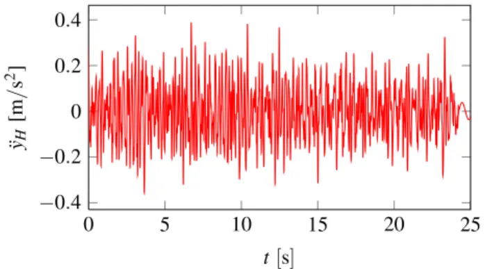
Figure 15. Lateral accelerations of the car body when the train crosses the viaduct at speedv=200 km/h.
0 2 4 6 8 10 12
−0.5 0 0.5
t[s]
¨
yH
[m
/
s
2 ]
Figure 16. Lateral accelerations of the car body when the train crosses the viaduct at speedv=350 km/h.
Determinaci´on de valores l´ımite(PT-2007-024-17CCP) and the Technical University of Madrid, Spain.
REFERENCES
[1] N Zhang, H Xia, and W Guo, “Vehicle-bridge interaction analysis under high-speed trains,”Journal of Sound and Vibration, vol. 309, no. 3-5, pp. 407–425, 2008.
[2] M Tanabe, H Wakui, N Matsumoto, H Okuda, M Sogabe, and S Komiya, “Computational model of a Shinkansen train running on the railway structure and the industrial applications,”Journal of Materials Processing Technology, vol. 140, no. 1-3, pp. 705–710, 2003.
[3] N Zhang, H Xia, W W Guo, and G De Roeck, “A VehicleBridge Linear Interaction Model and Its Validation,”International Journal of Structural Stability and Dynamics, vol. 10, no. 02, pp. 335, 2010.
[4] H Xia, N Zhang, and G D Roeck, “Dynamic analysis of high speed railway bridge under articulated trains,” Computers & Structures, vol. 81, pp. 2467–2478, 2003.
[5] H Xia and N Zhang, Dynamic Interaction of Vehicles and Structures, Science Press, Beijing, China, 2nd edition, 2005.
[6] D V Nguyen, K D Kim, and P Warnitchai, “Simulation procedure for vehicle-substructure dynamic interactions and wheel movements using linearized wheelrail interfaces,”Finite Elements in Analysis and Design, vol. 45, no. 5, pp. 341–356, 2009.
[7] D V Nguyen, K D Kim, and P Warnitchai, “Dynamic analysis of three-dimensional bridge-high-speed train interactions using a wheelrail contact model,”Engineering Structures, vol. 31, no. 12, pp. 3090–3106, 2009. [8] M K Song, H C Noh, and C K Choi, “New three-dimensional
finite element analysis model of high-speed train-bridge,” Engineering Structures, vol. 25, pp. 1611–1626, 2003.
[9] L Kwasniewski, H Li, J Wekezer, and J Malachowski, “Finite element analysis of vehicle-bridge interaction,” Finite Elements in Analysis and Design, vol. 42, no. 11, pp. 950–959, 2006.
[10] Y B Yang and J D Yau, “Vehicle-bridge interaction element for dynamic analysis,” Journal of Sound and Vibration, vol. 123, no. 11, pp. 1512– 1518, 1997.
[11] Y L Xu, N Zhang, and H Xia, “Vibration of coupled train and cable-stayed bridge systems in cross winds,” Engineering Structures, vol. 26, pp. 1389–1406, 2004.
[12] H Xia, Y M Cao, and N Zhang, “Numerical Analysis of Vibration Effects of Metro Trains on Surrounding Environment,” International Journal of Structural Stability and Dynamics, vol. 7, no. 1, pp. 151–166, 2007. [13] A A Shabana, K E Zaazaa, and H Sugiyama,Railroad Vehicle Dynamics:
A Computational Approach, CRC Press, 2008.
[14] K Popp and W Schiehlen, Ground Vehicle Dynamics, Springer Berlin Heidelberg, Chennai, 1st edition, 2010.
[15] Y S Wu and Y B Yang, “Steady-state response and riding comfort of trains moving over a series of simply supported bridges,” Engineering Structures, vol. 25, no. 2, pp. 251–265, 2003.
[16] J D Yau and Y B Yang, “Vibration reduction for cable-stayed bridges traveled by high-speed trains,” Finite Elements in Analysis and Design, vol. 40, pp. 341–359, 2004.
[17] N Zhang, H Xia, and W W Guo, “Spectrum and sensitivity analysis of vehicle-bridge interaction system,” inISEV’2007, Taipei, 2007, pp. 357– 362.
[18] H Hertz, “ ¨Uber die ber¨uhrung fester elasticher k¨orper and ¨uber die h¨artean,” J. f¨ur reine und agewandte Mathematik, vol. 92, pp. 156–171, 1882.
[19] J J Kalker, On the rolling contact of two elastic bodies in the presence of dry friction, Ph.D. thesis, Delft Unversity of Technology, 1967. [20] J J Kalker, “Book of tables for the Hertzian creep-force law,” in
Proceedings of the 2nd Mini Conference on Contact Mechanics and Wear of Wheel/Rail Systems, I Zobory, Ed., Budapest: Technical University of Budapest, 1996, pp. 11–20.
[21] J J Kalker, “The computation of three-dimensional rolling contact with dry friction,” International Journal for Numerical Methods in Engineering, vol. 14, no. 9, pp. 1293–1307, 1979.
[22] H Claus and W Schiehlen, “Modeling and Simulation of Railway Bogie Structural Vibrations,”Vehicle System Dynamics, vol. 29, no. 1, pp. 538– 552, Aug. 1997.
[23] G De Roeck, J Maeck, and A Teughels, “Train-bridge interaction: Validation of numerical models by experiments on high-speed railway bridge in Antoing,” inTIVC’2001, Beijing, 2001, pp. 283–294. [24] V K Garg and R V Dukkipati, Dynamics of Railway Vehicle Systems,
Academic Press, Ontario, 1984.
[25] H M Hilber, T J R Hughes, and R L Taylor, “Improved numerical dissipation for time integration algorithms in structural dynamics,”
Earthquake Engineering & Structural Dynamics, vol. 5, pp. 283–292, 1977.
[26] J J Kalker, Three-Dimensional Elastic Bodies in Rolling Contact (Solid Mechanics and Its Applications), Springer, 1990.