Trend analysis of CO
2
and CH
4
recorded at a semi-natural site in the
northern plateau of the Iberian Peninsula
Isidro A. P
erez
*, M. Luisa S
anchez, M.
Angeles García, Nuria Pardo
Department of Applied Physics, Faculty of Sciences, University of Valladolid, Paseo de Belen, 7, 47011 Valladolid, Spainh i g h l i g h t s
Four procedures were used to obtain the CO2and CH4trend and seasonal behaviour.
A time-dependent amplitude was considered in the harmonic equation.
Similar trends were obtained with the methods employed.
Kernel regression stands out among the nonparametric procedures used.
a r t i c l e i n f o
Article history: Received 30 June 2016 Received in revised form 28 November 2016 Accepted 29 November 2016 Available online 30 November 2016 Keywords:
Carbon dioxide Methane Long-term analysis Kernel smoothing Local regression
a b s t r a c t
CO2and CH4were recorded from October 2010 to February 2016 with a Picarro G1301 analyser at the centre of the upper plateau of the Iberian Peninsula. Large CO2values were observed during the vege-tation growing season, and were reinforced by the stable boundary layer during the night. Annual CH4 evolution may be explained by ecosystem activity and by the dispersion linked with the evolution of the boundary layer. Their trends were studied using an equation that considers one polynomial and one harmonic part. The polynomial part revealed an increasing trend from 0.8 to 2.3 ppm year1for CO2and from 0.004 to 0.011 ppm year1for CH4. The harmonic part considered four harmonics whose amplitudes were noticeable for thefirst and second harmonics for CO2and for thefirst harmonic for CH4. Long-term evolution was similar with alternative equations. Finally, seasonal study indicated summer minima for both gases, which may be explained by the lack of vegetation in this season. Harmonic analysis showed two maxima for CO2, one in spring linked with vegetation growth, which decreased with time, and another in autumn related with the onset of plant activity after the summer, which increased with time. CH4presented only one maximum in winter and a short time with steady concentration in spring where the evolution of the boundary layer may play a noticeable role. The harmonic equation, which takes into account all the observations, revealed opposite behaviour between CO2, whose minima decreased, and CH4, whose maxima increased.
©2016 Elsevier Ltd. All rights reserved.
1. Introduction
CO2and CH4are trace gases involved in the greenhouse effect
whose observations are continuously recorded worldwide (NOAA, 2016; WDCGG, 2016). Mauna Loa was the site where continuous measurements of atmospheric CO2commenced in 1958. Since this
year, the number of observatories has increased considerably. In particular, measurements started at certain stations during the nineties. In Europe, Vermeulen et al. (2011) have presented
measurements since 1993 at Cabauw in the Netherlands, andLohila et al. (2015)indicated that CO2has been measured since 1998 and
CH4since 2004 at Sammaltunturi, Finland. In North America, CO2
observations commenced in 1990 at the top of a 40-m tower at Fraserdale, Canada (Higuchi et al., 2003). This trace gas has been measured since 1992 on a 610-m tower in North Carolina and since 1994 on a 447-m tower in Wisconsin (Bakwin et al., 1998). In Asia,
Inoue et al. (2006)considered CO2recordings from a 200-m tower
at Tsukuba, Japan, from 1992. At Minamitorishima station, western North Pacific, these trace gases have been measured since 1993 (Wada et al., 2007), and CH4 measurements began at Waliguan,
China, in 1994 (Zhang et al., 2013).
CO2 natural sources are respiration processes and main *Corresponding author.
E-mail address:[email protected](I.A. Perez).
Contents lists available atScienceDirect
Atmospheric Environment
j o u r n a l h o m e p a g e : w w w . e l s e v i e r . c o m / l o c a t e / a t m o s e n v
http://dx.doi.org/10.1016/j.atmosenv.2016.11.068
anthropogenic sources are combustion of fossil fuels. The global anthropogenic emissions inventory of gaseous and particulate air pollutants, EDGAR, published by the European Commission revealed that the greatest emissions corresponded to China and the USA in 2014. Moreover, the increase in these global emissions almost stalled in that year. Specifically, they decreased from 4.1 to 3.4 billion tonnes between 2000 and 2014 in the European Union (Olivier et al., 2015). Natural sinks are the uptake by oceans and photosynthesis. As a result, CO2 atmospheric lifetime is 30e95
years (Jacobson, 2005). Its distribution over the globe presented concentrations around 400 ppm in the northern hemisphere in 2015, whereas they were slightly lower than this value in the southern hemisphere. Average seasonal evolution showed an accentuated cycle in the northern hemisphere with a maximum in winter-spring and a minimum in AugusteSeptember. Tropospheric CO2is increasing, its rate depending on ecosystem evolution and
measurement time, since observations indicate an irregular in-crease following the background concentration evolution (WMO, 2016). Hence, accurate determination of the CO2trend should be
obtained, since this also plays a useful role in investigating whether the control strategies for this gas's emissions are correct.
Initially, the current analysis takes an expression formed by one polynomial and one harmonic part, thefirst for the trend and the second part for seasonal behaviour. A specific part of this study is devoted to analysing the harmonic part. Although such an expression is frequently used, its detailed analysis is usually limited to amplitude, which is assumed constant in most of the research undertaken to date (Timokhina et al., 2015). The inclusion of time in the amplitude of the harmonic function is a major contribution made by the present research and provides a more in-depth anal-ysis of seasonal evolution.
Moreover, alternative procedures such as kernel regression, weighted linear regression and weighted quadratic regression are applied to investigate not only the long-term evolution but also the seasonal cycle, with their features, advantages, and drawbacks being discussed and compared.
CH4is another greenhouse gas whose behaviour has been less
widely studied to date. Anthropogenic sources are biomass burning, landfills, crops such as rice paddies and fossil fuel pro-duction and consumption. Natural sources are wetlands, oceans, geological seeps or enteric fermentation. Its main sink is oxidation by the hydroxyl radical (OH) in the troposphere, which means a lifetime of about 10 years. Its evolution over the globe may be observed fromWMO (2016). In 2015, its concentration was above 1.9 ppm for latitudes higher than 30 N, whereas it was below 1.8 ppm in the southern hemisphere. Seasonal evolution was slightly more accentuated in the Northern Hemisphere, where the maximum was reached in winter and the minimum in summer. Recently,Sanchez et al. (2014)investigated its directional behav-iour as well as daily and yearly cycles in the upper Spanish plateau, andGarcía et al. (2016)considered the influence of atmospheric stability and transport on its concentrations at the same site. In the current research, CH4analysis will run parallel to that of CO2.
2. Materials and methods
2.1. Experimental description
CO2and CH4dry concentrations were measured with a Picarro
G1301 at CIBA (Low Atmosphere Research Centre) 4148050.2700N, 455058.4400W, at 852 m above mean sea level. The measurements considered in this paper began on 15 October 2010 and extended to 29 February 2016. The analyser uses the wavelength-scanned cavity ringdown spectroscopy technique (Crosson, 2008) and achieves the WMO inter-laboratory comparability standard for both gases
without drying the sample gas (Chen et al., 2010; Rella, 2010; Rella et al., 2013). It was equipped with a valve sequencer to obtain ob-servations at 1.8, 3.7 and 8.3 m every 10 min at each level. Around 30 observations were taken each minute, although values were averaged every half an hour. Calibrations made every two weeks with three NOAA standards revealed the extreme stability of the device and were used to slightly correct observations applying the following linear equations (in ppm):
CO2C¼1:00341CO20:17870 (1)
CH4C¼0:99197CH4þ0:01249 (2)
where theCsubscript denotes the corrected value.
2.2. Harmonic regression
The CO2 time series may be considered to comprise three
components, the trend component, the seasonal component and the remainder component (Cleveland et al., 1990). One initial problem concerns the separation between the seasonal cycle and the long-term evolution. Thoning and Tans (1989) introduced a digital filtering technique to achieve this objective. However, simpler alternative procedures have successfully been considered. At Lampedusa,Artuso et al. (2009)used an exponential function to describe the long-term CO2trend whosefit is not possible by linear
regression. Measurements reveal that this trend is not affected by sharp changes and may be approximated by a linear term (Chamard et al., 2003), which is usually extended to a polynomial equation.
The current analysis is based on the procedure presented by
Nakazawa et al. (1997), which used an equation with polynomial and harmonic parts similar to
y¼X3 i¼0
aitiþX4 j¼1
X1 k¼0
bjktk cosðj2
p
tÞ þcjktk sinðj2
p
tÞ(3)
This equation is taken as a reference since it has often been used in similar studies, such asBakwin et al. (1998)orFang et al. (2016).
Eneroth et al. (2005)andInoue et al. (2006)used equations with three harmonics. However, this paper considers four harmonics, in agreement with Tans et al. (1989) and Vermeulen et al. (2011), although both analyses evidence a linear trend. However, the main contribution of equation(3)is the time affecting the amplitude. In our case,yis CO2or CH4concentrations andtis the time measured
in years.
Equation(3)is proposed to describe the global evolution by the polynomial part and the evolution of the yearly cycle by the har-monic part. First and second harhar-monics are related with the yearly cycle, since thefirst harmonic proposes times and values for the yearly maxima and minima and the second corrects or reinforces them. However, the remaining harmonics considered focus on the seasonal pattern. Consequently, shorter time intervals are not taken into account by Eq.(3).
In the case of a slow time variation in the amplitude of each frequency, Eq.(3)may be written as
y¼X3 i¼0
aitiþX4 j¼1
AjðtÞcos 2
p
tTj
q
j !(4)
where amplitude Aj(t), period Tjand phase constant
q
jmust bedetermined experimentally. For each frequencyjof Eq.(3), theN
maxima of the harmonic part are determined,Yj1…YjN. The time
between consecutive maxima,tjiþ1-tji, is one period, resulting in
must be null for every maximum of Eq.(4), the phase constant,
q
ji,may be obtained from each timetjicorresponding to maximaYji. In
order to avoid the discontinuity of this angular variable at 0,
q
jishould be treated as a vector and its components, cos
q
jiand sinq
ji,should be calculated and averaged to obtain the mean phase con-stant,
q
j.Finally, amplitude is calculated by linear interpolations between consecutive maxima and extrapolations at the edges, before the first maximum and beyond the last maximum.
AjðtÞ ¼ 8 > > > > > > > > > < > > > > > > > > > :
Yj1þYj2Yj1 tj2tj1
ttj1if t<tj1
Yjiþ
Yjiþ1Yji tjiþ1tji
ttji
if tji<t<tjiþ1
YjN1þ
YjNYjN1 tjNtjN1
ttjN1
if tjN<t
(5)
2.3. Kernel regression
This is a weighted mean calculated by
yðt;hÞ ¼
PN i¼1K
tti h yi PN i¼1 tti h (6)
wheretis the time when the concentrationyis calculated,yiare
experimental values of concentration at ti, h is the width of a
window and K is the kernel function. The Gaussian kernel has sometimes been used (Donnelly et al., 2011), since it includes all observations. However, the extremely long time required to make the calculations when many observations are involved has led to it being replaced by the Epanechnikov kernel,
K
tti h
¼0:75 1
tti
h 2!
;1tti
h 1 (7)
which was also used in this kind of calculations (Henry et al., 2002). Only observationstiranging fromt-htotþh are considered in this
kernel.
The procedure followed in this paper was based onGraven et al. (2012). Observations werefirst detrended with a wide window, and seasonal cycles were considered by smoothing the detrended ob-servations with a narrow window. Finally, these seasonal cycles were subtracted from the original observations and the resulting series was smoothed again with the initial window. The narrow window was 60 days so as to consider seasonal changes, whereas a test was conducted to choose the wide window with values from 300 to 1000 days in 100-day intervals. Oscillations disappeared with a 500-day window, which was the value selected.
A noticeable feature of this procedure is that only half the ob-servations take part in calculations at the beginning or end of the measurement period.
2.4. Other nonparametric procedures
Some local regression methods were suggested byCleveland (1979)andCleveland and Devlin (1988)to obtain visual informa-tion from a scatterplot.
The tri-cube weight function is usually employed. However, weights are calculated in this paper employing the Epanechnikov
kernel to use the same weight function in the procedures pre-sented. Two methods were followed: thefirst considers a weighted linear regression, y ¼a0 þ a1t, whose coefficients were easily
calculated by
a1¼
Pq i¼1wi
titw
yiyw
Pq i¼1wi
titw
2 (8)
a0¼ywa1tw (9)
wherewiare the weights andtwandyware obtained from
tw¼
Pq i¼1witi Pq
i¼1wi
(10)
yw¼
Pq i¼1wiyi Pq
i¼1wi
(11)
and the second used a weighted quadratic regression,
y¼b0þb1tþb2t2. The coefficient calculation is given by
b¼XTWX 1
XTWy (12)
where y is the matrix of the response variable, which is the observed concentration,Wis the diagonal matrix containing the weights, and the matricesXandbare
X¼
0 B B @
1 t1 t2 1
1 t2 t22 / / /
1 tn tn2 1 C C A;b¼
0 @bb01
b2
1
A (13)
3. Results
Calculations for the harmonic model were made in Matlab since this easily handles multiple linear regressions in addition to which the time employed was short. Its main advantage is that trend calculation and seasonal behaviour analysis are carried out in a single step. The remaining calculations were made in Fortran, with the calculation time being noticeably long for the weighted quadratic regression.
3.1. CO2and CH4variation
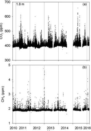
Availability of observations was around 84% due to noticeable gaps in August 2013 and 2015, and from August to the end of 2014. CO2median concentration was 401.5 ppm for the 1.8-m level, with
an interquartile range of 11.9 ppm. For the 8.3-m level, concentra-tion was 0.6 ppm lower and the interquartile range 1.6 ppm nar-rower. Observations for the lowest level are presented inFig. 1(a) where the seasonal pattern is revealed by noticeable values in spring and low values in summer. Large measurements could be explained by plant respiration during the growing season together with the formation of a stable boundary layer during the night. Occasional emissions from vehicles used in farming around the site should not be excluded. However, the low values observed in summer may be attributed to the lack of vegetation in this season. For CH4, median concentration was 1.899 ppm at the lowest
level, with an interquartile range of 0.040 ppm, whereas concen-tration was 0.001 ppm higher with similar interquartile range for I.A. Perez et al. / Atmospheric Environment 151 (2017) 24e33
the highest level. Its seasonal cycle is much less marked since measurements are located in a very narrow interval,Fig. 1(b). The largest values were recorded in winter when soil and plant activ-ities increase due to the rains and the low values of the boundary layer height are also reached.
3.2. Harmonic regression
Fig. 2presents the results of Eqs.(3)e(4)for the lowest level, since the changes are more pronounced for CO2than in the other
levels. Both gases present an increasing trend with rapid growth over the latter years. The main advantage of this procedure is that the lack of data does not prevent calculations from continuing since this methodfills in the gaps.
Following those equations, the CO2yearly cycle is described by a
maximum in spring linked with the development of vegetation activity, which was noticeable in 2011 but moderate in 2015. A second maximum was observed in autumn, which was attributed to soil and plant activities with thefirst rains after summer. The contribution of this maximum was slight in 2011, but gradually increased and was noticeable in 2015. The CO2 minimum was
reached in summer, when vegetation almost vanishes. Concentra-tion at this time also increased from 2011 to 2015, although the CO2
hole was deeper in 2015 than in 2011.
The CH4 yearly cycle was simpler than that for CO2. Maxima
were observed in winter, whereas minima were found in summer. Moreover, a short period with a steady concentration was observed in spring. In agreement with CO2, the increase was faster at the end
than at the beginning of the period analysed.
Agreement of Eq.(3)was described by R2, which was between 0.14 and 0.28 for CO2at the lowest and highest levels, respectively,
and around 0.10 for CH4. These low values are attributed to the
noticeable daily changes of the half hour means that were used.
When daily means are considered, values are steadier and R2 in-creases, extending from 0.40 to 0.59 for CO2, whereas it remained
around 0.30 for CH4. Finally, when monthly means are used, R2
ranged from 0.87 to 0.93 for CO2and was around 0.89 for CH4.
Moreover,Fig. (2)shows the satisfactory agreement between Eqs.
(3) and (4).
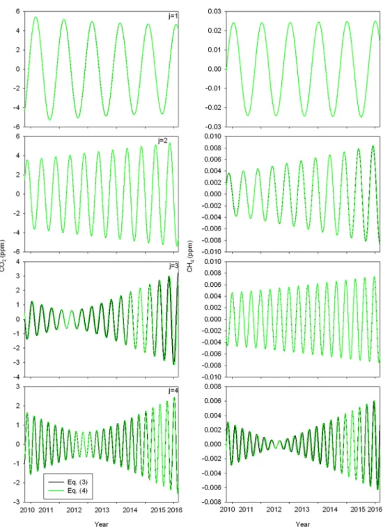
Fig. 3shows the four harmonics calculated with Eqs.(3) and (4). Two amplitude groups may be observed. For CO2, thefirst group is
formed by thefirst and second harmonics, whose greatest ampli-tudes were slightly below 6 ppm. The second group comprises the third and fourth harmonics, with amplitudes reaching around 3 ppm. For CH4, thefirst group is formed by thefirst harmonic,
whose amplitude was around 0.025 ppm, whereas the remaining harmonics make up a second group whose amplitude is around 0.008 ppm at most.
Thefirst harmonic amplitude decreased slightly with time for CO2, and increased for the CO2second harmonic and from thefirst
to third harmonics of CH4. In these cases, Eq.(5)may be simplified
by a linear relationship. The remaining harmonics displayed a more complex evolution with a decreasing trend in the amplitude at the beginning of the period considered and an increasing trend at the end, reaching a minimum in 2012. The contribution of the first harmonic is almost time independent for both trace gases, whereas the fourth harmonic was noticeably small for CH4in 2012.
Fig. 3reveals that the addition of two harmonic functions, one with constant amplitude and the second whose amplitude changes slowly with time, results in a harmonic function whose amplitude changes slowly with time: hence the satisfactory agreement be-tween the harmonic parts of Eqs.(3) and (4).
Fig. 1.Observations (half hour averages) for the lowest level considered in the current
analysis. Fig. 2.Evolution for CO2(a) and CH4(b) obtained with Eqs.(3) and (4), which are
formed by a polynomial part and a harmonic part.
3.3. Trend analysis
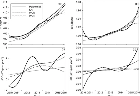
Fig. 4presents the evolutions of both trace gases together with their growth rate. CO2concentration increased 12.3 ppm during the
measurement period for the polynomial part that reveals the trend in Eq.(3). The trend average value was 1.7 ppm year1. However, this increase was not regular since at the end of 2010 the growth rate was low, around 0.8 ppm year1whilst, contrastingly, the trend reached 2.3 ppm year1in early 2016.
For CH4, the increase was 0.059 ppm, with an average of
0.006 ppm year1. Its growth rate began at nearly 0.004 ppm year1 andfinished at 0.011 ppm year1. This polynomial evolution was considered a reference since equations similar to Eq. (3) are
frequently used.
Alternative procedures showed a similar evolution. The poly-nomial model determined the steadiest trend. However, small os-cillations were observed when the weighted quadratic regression was used. The greatest discrepancies for CH4 observed at the
beginning and end of the measurement period for this latter method could be attributed to a border effect, since calculations were made with half the observations in the window. Thefl uctu-ating behaviour of the weighted quadratic regression was notice-able in the growth rate displayed in the lower plots of thisfigure and is due to the width of the wide window used, i.e. 500 days, which was considered to compare the procedures in similar con-ditions. When using a wider window, such as 1000 days, Fig. 3.CO2and CH4concentrations calculated by the four harmonics used in Eqs.(3) and (4).
oscillations disappear.
Fig. 5shows the seasonal evolution formed by the harmonic part of Eq.(3)and once the observations were detrended in the other methods. Spring and autumn CO2maxima were noticeable in the
harmonic equation. However, the summer CO2minima decreased
markedly with time despite the lack of observations in August from 2013 to 2015. Moreover, winter CH4maxima increased with time.
Seasonal evolution for the kernel regression and weighted linear regression were very similar and revealed noticeable discrepancies with the harmonic evolution of both trace gases, mainly during the latter years of the period considered. Oscillation was softer than observed with the harmonic equation for CO2, and winter maxima
were smaller for CH4. However, weighted quadratic regression
provided values close to those of the harmonic evolution. Finally, the harmonic equation provided more regular changes and, in some way, proves lessflexible than the other procedures that describe better the changes observed in relatively short times determining an irregular evolution.
4. Discussion
4.1. Observations
The CO2evolution presented inFig. 1is similar to that observed
at different places. The lowest concentration was close to 400 ppm. Similar values were observed at Lin'an, China for the period 2009e2011 (Pu et al., 2014). However,Hernandez-Paniagua et al. (2015) presented observations at southwest London where the lowest values were smaller, even reaching 350 ppm in the period 2000e2002. Similarly, the lowest values of CO2 concentration at
Cabaw, the Netherlands, were below 380 ppm (Vermeulen et al., 2011). The highest concentration at CIBA was occasionally above 500 ppm.Zhu and Yoshikawa-Inoue (2015)observed large episodic high CO2events during summer on Rishiri Island, western North
Pacific, which were attributed to high emissions from local soil and vegetation and the stable nocturnal boundary layer. High values
reached in spring at CIBA may have a similar origin, although some might be due to vehicles used in farming. The opposite behaviour was observed at Lin'an, where the highest values were more moderate. CH4measured at CIBA was confined at a narrow interval
determined by the interquartile range, 0.040 ppm. Although the lowest values were similar to those observed at Cabaw, they were mainly located over a wider interval during the period 2000e2010.
4.2. Trend analysis
The range of trends presented inTable 1is very wide since it extends 2.5 ppm year1.Wu et al. (2012)obtained the same value as that observed at CIBA, 1.7 ppm year1, which is close to the global average of the last decade, nearly 2.1 ppm year1(WMO, 2016). This trend was similar in Mauna Loa, where it has been above 2.0 ppm year1in recent years (Hofmann et al., 2009). The increase at the beginning of the measurement period was smaller than values presented in Table 1, whose lowest trend was 1.3 ppm year1at a site in Antarctica. However, at the end of the measurement period the trend was similar to Egham, UK, or Pallas, Finland, although far from the highest, which was 3.8 ppm year1, observed in China.
Since interactions between natural and anthropogenic pro-cesses are complex, positive feedback in the biosphere determines the CO2increase. Among global scope processes, El Nino-Southern~
Oscillation is correlated with variations in the CO2 growth rate
(Heimann and Reichstein, 2008; Ruzmaikin et al., 2012). Moreover, different studies reveal that CO2uptake by terrestrial ecosystems
(carbon sink) influences atmospheric CO2concentrations.Ahlstrom€ et al. (2015) concluded that semi-arid ecosystems dominate the trend and inter-annual variability of the sink. The role of winter snow in the northern forest merits further research since the decrease in winter respiration justifies the carbon sink enhance-ment (Yu et al., 2016). Additionally, observations over the last sixty years indicate that CO2uptake is stimulated during spring, while an
earlier release of CO2into the atmosphere was observed in autumn Fig. 4.Trends of CO2(a) and CH4(b) together with their corresponding growth rates, (c) and (d), for polynomial, kernel regression (KR), weighted linear regression (WLR) and
weighted quadratic regression (WQR).
at latitudes above 45 N (Barichivich et al., 2013). Finally, un-certainties remain in the magnitude and sign of CO2sink trends
(Sitch et al., 2015), and future studies should consider the effects of nonlinear interactions of dominant drivers on the trend of land carbon uptake (Zhang et al., 2016).
WMO (2016) presented growth rates for CH4 in the range
0.005e0.010 ppm year1in recent years, which might partially be explained by the global impact of the increase in anthropogenic emissions in Asia (Dalsøren et al., 2016).Bergamaschi et al. (2013)
described a growth rate peak of about 0.01 ppm year1in early 2007, preceded by a nearly null growth rate during 2005 and fol-lowed by slow attenuation. Vermeulen et al. (2011) provided a reference value of 0.0059 ppm year1for the period 2005e2010, which was similar to the value at CIBA, and a rate of 0.0074 ppm year1at Cabaw, the Netherlands (Table 2). The most noticeable trend presented in this table, about 0.050 ppm year1, was observed at Hegyhatsal, Hungary, although it corresponded to a short period, 2007e2009.
Increased emissions in the tropical and mid-latitude Northern Hemisphere are considered to be responsible for the CH4increase
since 2007 (Nisbet et al., 2014), which may be explained by the increase in emissions from natural wetlands, fossil fuel-related emissions or the decrease in OH concentrations (Sussmann et al., 2012). Moreover, the current network does not allow a descrip-tion of emissions by region and source processes and attributing this increase to natural and anthropogenic sources is not easy since emissions from both sources are superimposed (Bergamaschi et al., 2013). Additionally, the global scale of different processes should not be ignored.Ginzburg et al. (2011)considered the influence of the winter of 2006e2007, which was anomalously warm in northern Europe and western Siberia, on the CH4increase recorded
in 2007. Similarly, anthropogenic emissions in Asia seem to have a global impact although their timing or strength has been ques-tioned (Dalsøren et al., 2016).
4.3. Harmonic analysis
Sanchez et al. (2010)considered CO2 evolution at CIBA from
February 2000 to December 2008 by means of a simple harmonic model with two harmonics (for the yearly and half-yearly cycles), although only the yearly cycle presented variable amplitude. The half-yearly cycle was evident during thefirst years. However, the
yearly cycle prevailed at the end. Yearly amplitude increased by 0.65 ppm year1. This value was similar to that provided by Eq.(3), Fig. 5.Seasonal evolution of CO2(a) and CH4(b) for the harmonic equation, kernel
regression (KR), weighted linear regression (WLR) and weighted quadratic regression (WQR).
Table 1
CO2trend and harmonic equations used in different studies.
Reference Site Trend (ppm year1) Period Polynomial part Harmonic part
Aalto et al. (2002) Pallas, Finland 2.5 1996e2000 Linear Three harmonics
Artuso et al. (2009) Lampedusa, Italy 1.9 1992e2007 Two harmonics
Bakwin et al. (1998) Eastern North Carolina 1992e1997 Second order Four harmonics
Northern Wisconsin 1994e1997
Cundari et al. (1995) Mt. Cimone, Italy 1.66 1979e1991
Eneroth et al. (2005) Pallas, Finland 1997e2003 Linear Three harmonics
Fang et al. (2016) Shangdianzi, China 2.7e3.8 2009e2013 Second order Four harmonics
Hernandez-Paniagua et al. (2015) Egham, UK 2.45 2000e2012
Mace Head, Ireland 1.9 2000e2011
Inoue et al. (2006) Tsukuba, Japan 2.0 1992e2003 Fourth order Three harmonics
Jain et al. (2005) Maitri (Antarctica) 1.3 2002e2003
Liu et al. (2015) Different sites in the Northern Hemisphere 2.04 1997e2006 Linear One harmonic
McClure et al. (2016) Mt. Bachelor, Oregon 1.48 2012e2014
Tans et al. (1989) Point Barrow, Alaska 1.44 1983e1985 Linear Four harmonics
Timokhina et al. (2015) Central Siberia, Russia 2.02 2006e2013 Linear Four harmonics
Vermeulen et al. (2011) Cabaw, The Netherlands 2.00 2005e2009 Linear Four harmonics
Wu et al. (2012) Northeast China 1.7 2003e2010 Linear One harmonic
Zhang et al. (2008) Seven sites in China 1.7e3.6 2003e2006
which was 0.55 ppm year1for the lowest level.
Wu et al. (2012)considered only one harmonic with a variable amplitude to investigate CO2evolution in a tall forest in China, this
reaching an increase in the seasonal cycle of 0.58 ppm year1and which was explained from measurements at Mauna Loa, Hawaii, by the biosphere's seasonal CO2“inhalations”and“exhalations”that
have become more pronounced. Moreover, Arctic Oscillation led to an early spring and to higher winter temperatures, resulting in increased seasonal amplitudes.
Liu et al. (2015)presented CO2evolution over nine ecosystems
in the period 1997e2006. They used only one harmonic with a variable amplitude. Concentrations seemed steady in three of them. Amplitude remained steady or increased slightly in four ecosys-tems, increasing clearly in three and decreasing in one. The amplitude in the last ecosystemfirst decreased, although it then increased after one very low value.
4.4. Seasonal cycle
The yearly behaviour for CO2described inFig. 5responds to the
average seasonal cycle fromWMO (2016). However, spring and autumn maxima are more marked inFig. 5since this plot corre-sponds to a specific site. Moreover, thisfigure is in agreement with that reported byCundari et al. (1995), who presented the seasonal evolution in 1989 at Mt. Cimone, although the spring maximum was barely visible and a noticeable scatter of measurements was observed in summer. Such a cycle with two maxima was also described byHatakka et al. (2003)for CO2concentration at Pallas,
Finland, from 1997 to 2003.
Climate-vegetation-carbon cycle feedback is noticeable above 40N. The seasonal CO2cycle has become more marked since the
1960s although the underlying mechanisms are not yet fully known (Forkel et al., 2016). The decreasing summer minima could be attributed to an increase in vegetation photosynthetic activity during the growing season (Angert et al., 2005). Similarly,
Barichivich et al. (2013)concluded that the long term increase in the amplitude of the CO2annual cycle above 45N over Eurasia is
associated with the lengthening and intensification of the photo-synthetic growing season.
A similar evolution to that observed for CH4 at CIBA was
re-ported byPickers and Manning (2015)at the Alert Station in Canada and byVermeulen et al. (2011)at Cabaw in the Netherlands where, in addition, a steady concentration was observed in spring. Although oxidation by OH contributes to the minimum obtained in summer, dispersive processes linked with the development of the boundary layer should not be ignored. Since observations of this variable are not available, the temperature at Valladolid, obtained fromAEMET (2016), may be used instead. In winter, temperature is low and the boundary layer is barely developed, causing high concentration values. In summer, thermal turbulence was intense and produced well developed boundary layers, with low concen-trations being observed. Temperature decrease from summer to winter is rapid. However, the temperature increase from winter to summer presents a period with steady values in spring, which may be linked to intermediate boundary layer heights and steady
concentrations. However, in Waliguan, China, the annual pattern was the opposite, with one minimum in spring and winter and one maximum in summer. This specific evolution may be explained by regional and local sources together with the dominant airflow from polluted regions in summer (Zhang et al., 2013).
5. Conclusions
Amplitudes of thefirst and second harmonics are noticeable for CO2, whereas only thefirst harmonic is enough for CH4. These
amplitudes present a linear evolution with time in the period October 2010eFebruary 2016.
Trend calculation shows slight differences following the pro-cedure used. Although the addition of polynomial and harmonic parts is common, alternative methods, such as kernel regression, may be successfully employed.
Trend increased for both trace gases with the different proced-ures used. However, seasonal analysis with the harmonic equation revealed an unequal trend for both gases, with minima decreasing for CO2 and maxima increasing for CH4. This behaviour may be
because all observations are considered, whereas the rest of the methods used only local neighbouring observations when calculating.
Since small changes are observed not only in the trend but also in the yearly cycle of both trace gases, procedure selection should be guided by the simplicity of the formulation and by calculation speed. Taking into account these features, kernel regression pro-vides fast and accurate values to determine the evolution of both trace gases for the trend and inside the yearly cycle.
Although the analysis presented in the current paper involved concentrations recorded at a semi-natural site, the influence of air mass trajectories on concentrations and their trends should be considered for a more accurate description of the evolution of both trace gases.
Conflict of interests
The authors declare that there is no conflict of interests regarding publication of this paper.
Acknowledgements
The authors wish to acknowledge thefinancial support of the Ministry of Economy and Competitiveness and ERDF funds (pro-jects CGL2009-11979 and CGL2014-53948-P).
References
Aalto, T., Hatakka, J., Paatero, I., Tuovinen, J.P., Aurela, M., Laurila, T., Holmen, K., Trivett, N., Viisanen, Y., 2002. Tropospheric carbon dioxide concentrations at a northern boreal site in Finland: basic variations and source areas. Tellus, Ser. B Chem. Phys. Meteorol. 54, 110e126.
AEMET (Agencia Estatal de Meteorología), 2016.http://www.aemet.es/es/portada. Accessed, September 2016.
Ahlstr€om, A., Raupach, M.R., Schurgers, G., Smith, B., Arneth, A., Jung, M., Reichstein, M., Canadell, J.G., Friedlingstein, P., Jain, A.K., Kato, E., Poulter, B., Sitch, S., Stocker, B.D., Viovy, N., Wang, Y.P., Wiltshire, A., Zaehle, S., Zeng, N., Table 2
CH4trend and harmonic equations used in different studies.
Reference Site Trend (ppm year1) Period Polynomial part Harmonic part
Fang et al. (2016) Shangdianzi, China 0.006e0.010 2009e2013 Second order Four harmonics
Haszpra et al. (2011) Hegyhatsal, Hungary 0.050 2007e2009
Nisbet et al. (2014) Globally averaged 0.006 2007e2013
Pedersen et al. (2005) Mt. Zeppelin, Norway 0.00334e0.00363 1998e2005
Vermeulen et al. (2011) Cabaw, The Netherlands 0.0074 2005e2010 Linear Four harmonics
2015. The dominant role of semi-arid ecosystems in the trend and variability of the land CO2sink. Science 348, 895e899.
Angert, A., Biraud, S., Bonfils, C., Henning, C.C., Buermann, W., Pinzon, J., Tucker, C.J., Fung, I., 2005. Drier summers cancel out the CO2uptake enhancement induced by warmer springs. Proc. Natl. Acad. Sci. U. S. A. 102, 10823e10827.
Artuso, F., Chamard, P., Piacentino, S., Sferlazzo, D.M., De Silvestri, L., di Sarra, A., Meloni, D., Monteleone, F., 2009. Influence of transport and trends in atmo-spheric CO2at Lampedusa. Atmos. Environ. 43, 3044e3051.
Bakwin, P.S., Tans, P.P., Hurst, D.F., Zhao, C., 1998. Measurements of carbon dioxide on very tall towers: results of the NOAA/CMDL program. Tellus, Ser. B Chem. Phys. Meteorol. 50, 401e415.
Barichivich, J., Briffa, K.R., Myneni, R.B., Osborn, T.J., Melvin, T.M., Ciais, P., Piao, S., Tucker, C., 2013. Large-scale variations in the vegetation growing season and annual cycle of atmospheric CO2at high northern latitudes from 1950 to 2011. Glob. Change Biol. 19, 3167e3183.
Bergamaschi, P., Houweling, S., Segers, A., Krol, M., Frankenberg, C., Scheepmaker, R.A., Dlugokencky, E., Wofsy, S.C., Kort, E.A., Sweeney, C., Schuck, T., Brenninkmeijer, C., Chen, H., Beck, V., Gerbig, C., 2013. Atmospheric CH4in thefirst decade of the 21st century: inverse modeling analysis using SCIAMACHY satellite retrievals and NOAA surface measurements. J. Geophys. Res. D. Atmos. 118, 7350e7369.
Chamard, P., Thiery, F., Di Sarra, A., Ciattaglia, L., De Silvestri, L., Grigioni, P., Monteleone, F., Piacentino, S., 2003. Interannual variability of atmospheric CO2 in the Mediterranean: measurements at the island of Lampedusa. Tellus, Ser. B Chem. Phys. Meteorol. 55, 83e93.
Chen, H., Winderlich, J., Gerbig, C., Hoefer, A., Rella, C.W., Crosson, E.R., Van Pelt, A.D., Steinbach, J., Kolle, O., Beck, V., Daube, B.C., Gottlieb, E.W., Chow, V.Y., Santoni, G.W., Wofsy, S.C., 2010. High-accuracy continuous airborne measure-ments of greenhouse gases (CO2and CH4) using the cavity ring-down spec-troscopy (CRDS) technique. Atmos. Meas. Tech. 3, 375e386.
Cleveland, R.B., Cleveland, W.S., McRae, J.E., Terpenning, I., 1990. STL: a seasonal-trend decomposition procedure based on loess. J. Off. Stat. 6, 3e73.
Cleveland, W.S., 1979. Robust locally weighted regression and smoothing scatter-plots. J. Am. Stat. Assoc. 74, 829e836.
Cleveland, W.S., Devlin, S.J., 1988. Locally weighted regression: an approach to regression analysis by localfitting. J. Am. Stat. Assoc. 83, 596e610.
Crosson, E.R., 2008. A cavity ring-down analyzer for measuring atmospheric levels of methane, carbon dioxide, and water vapor. Appl. Phys. B 92, 403e408.
Cundari, V., Colombo, T., Ciattaglia, L., 1995. Thirteen years of atmospheric carbon dioxide measurements at Mt. Cimone station. Italy. Il Nuovo Cimento C 18, 33e47.
Dalsøren, S.B., Myhre, C.L., Myhre, G., Gomez-Pelaez, A.J., Søvde, O.A., Isaksen, I.S.A., Weiss, R.F., Harth, C.M., 2016. Atmospheric methane evolution the last 40 years. Atmos. Chem. Phys. 16, 3099e3126.
Donnelly, A., Misstear, B., Broderick, B., 2011. Application of nonparametric regression methods to study the relationship between NO2concentrations and local wind direction and speed at background sites. Sci. Total Environ. 409, 1134e1144.
Eneroth, K., Aalto, T., Hatakka, J., Holmen, K., Laurila, T., Viisanen, Y., 2005. Atmo-spheric transport of carbon dioxide to a baseline monitoring station in northern Finland. Tellus, Ser. B Chem. Phys. Meteorol. 57, 366e374.
Fang, S.X., Tans, P.P., Dong, F., Zhou, H., Luan, T., 2016. Characteristics of atmospheric CO2and CH4at the Shangdianzi regional background station in China. Atmos. Environ. 131, 1e8.
Forkel, M., Carvalhais, N., Rodenbeck, C., Keeling, R., Heimann, M., Thonicke, K.,€ Zaehle, S., Reichstein, M., 2016. Enhanced seasonal CO2exchange caused by amplified plant productivity in northern ecosystems. Science 351, 696e699.
García, M.A., Sanchez, M.L., Perez, I.A., Ozores, M.I., Pardo, N., 2016. Influence of atmospheric stability and transport on CH4concentrations in northern Spain. Sci. Total Environ. 550, 157e166.
Ginzburg, A.S., Vinogradova, A.A., Fedorova, E.I., 2011. Some features of seasonal variations in the methane content in the atmosphere over northern Eurasia. Izv. Atmos. Ocean. Phys. 47, 45e58.
Graven, H.D., Guilderson, T.P., Keeling, R.F., 2012. Observations of radiocarbon in CO2
at La Jolla, California, USA 1992-2007: analysis of the long-term trend. J. Geophys. Res. D. Atmos. 117, D02302.http://dx.doi.org/10.1029/2011JD016533. Haszpra, L., Barcza, Z., Szilagyi, I., Dlugokencky, E., Tans, P., 2011. Trends and tem-poral variations of major greenhouse gases at a rural site in central Europe. In: L. Haszpra (Ed.). Atmospheric Greenhouse Gases: the Hungarian Perspective, pp. 29e47.
Hatakka, J., Aalto, T., Aaltonen, V., Aurela, M., Hakola, H., Komppula, M., Laurila, T., Lihavainen, H., Paatero, J., Salminen, K., Viisanen, Y., 2003. Overview of the at-mospheric research activities and results at Pallas GAW station. Boreal Environ. Res. 8, 365e383.
Heimann, M., Reichstein, M., 2008. Terrestrial ecosystem carbon dynamics and climate feedbacks. Nature 451, 289e292.
Henry, R.C., Chang, Y.S., Spiegelman, C.H., 2002. Locating nearby sources of air pollution by nonparametric regression of atmospheric concentrations on wind direction. Atmos. Environ. 36, 2237e2244.
Hernandez-Paniagua, I.Y., Lowry, D., Clemitshaw, K.C., Fisher, R.E., France, J.L., Lanoiselle, M., Ramonet, M., Nisbet, E.G., 2015. Diurnal, seasonal, and annual trends in atmospheric CO2at southwest London during 2000-2012: wind sector analysis and comparison with Mace Head. Irel. Atmos. Environ. 105, 138e147.
Higuchi, K., Worthy, D., Chan, D., Shashkov, A., 2003. Regional source/sink impact on the diurnal, seasonal and inter-annual variations in atmospheric CO2at a boreal
forest site in Canada. Tellus, Ser. B Chem. Phys. Meteorol. 55, 115e125.
Hofmann, D.J., Butler, J.H., Tans, P.P., 2009. A new look at atmospheric carbon di-oxide. Atmos. Environ. 43, 2084e2086.
Inoue, H.Y., Matsueda, H., Igarashi, Y., Sawa, Y., Wada, A., Nemoto, K., Sartorius, H., Schlosser, C., 2006. Seasonal and long-term variations in atmospheric CO2and 85Kr in Tsukuba, central Japan. J. Meteorol. Soc. Jpn. 84, 959e968.
Jacobson, M.Z., 2005. Erratum:“Control of fossil-fuel particulate black carbon and organic matter, possibly the most effective method of slowing global warming”. J. Geophys. Res. D. Atmos. 110, 1e5.
Jain, S.L., Ghude, S.D., Kumar, A., Arya, B.C., Kulkarni, P.S., 2005. Continuous obser-vations of surface air concentration of carbon dioxide and methane at Maitri. Antarct. Curr. Sci. 88, 1941e1948.
Liu, M., Wu, J., Zhu, X., He, H., Jia, W., Xiang, W., 2015. Evolution and variation of atmospheric carbon dioxide concentration over terrestrial ecosystems as derived from eddy covariance measurements. Atmos. Environ. 114, 75e82.
Lohila, A., Penttil€a, T., Jortikka, S., Aalto, T., Anttila, P., Asmi, E., Aurela, M., Hatakka, J., Hellen, H., Henttonen, H., H€anninen, P., Kilkki, J., Kyll€onen, K., Laurila, T., Lepisto, A., Lihavainen, H., Makkonen, U., Paatero, J., Rask, M., Sutinen, R.,€ Tuovinen, J.P., Vuorenmaa, J., Viisanen, Y., 2015. Preface to the special issue on integrated research of atmosphere, ecosystems and environment at Pallas. Boreal Environ. Res. 20, 431e454.
McClure, C.D., Jaffe, D.A., Gao, H., 2016. Carbon dioxide in the free troposphere and boundary layer at the Mt. Bachelor observatory. Aerosol Air Qual. Res. 16, 717e728.
Nakazawa, T., Ishizawa, M., Higuchi, K., Trivett, N.B.A., 1997. Two curvefitting methods applied to CO2flask data. Environmetrics 8, 197e218.
Nisbet, E.G., Dlugokencky, E.J., Bousquet, P., 2014. Methane on the rise - again. Science 343, 493e495.
NOAA (National Oceanic and Atmospheric Administration, 2016. Global Monitoring Division.http://www.esrl.noaa.gov/gmd/. Accessed, September 2016. Olivier, J.G.J., Janssens-Maenhout, G., Muntean, M., Peters, J.H.A.W., 2015. Trends in
Global CO2Emissions - 2015 Report, JRC Report 98184/PBL Report 1803.http:// edgar.jrc.ec.europa.eu/overview.php?v¼CO2ts1990-2014. Accessed, September 2016.
Pedersen, I.T., Holmen, K., Hermansen, O., 2005. Atmospheric methane at zeppelin station in Ny-Ålesund: Presentation and analysis of in situ measurements. J. Environ. Monit. 7, 488e492.
Pickers, P.A., Manning, A.C., 2015. Investigating bias in the application of curve fitting programs to atmospheric time series. Atmos. Meas. Tech. 8, 1469e1489.
Pu, J.J., Xu, H.H., He, J., Fang, S.X., Zhou, L.X., 2014. Estimation of regional background concentration of CO2at Lin'an station in Yangtze river delta, China. Atmos. Environ. 94, 402e408.
Rella, C., 2010. Accurate Greenhouse Gas Measurements in Humid Gas Streams Using the Picarro G1301 Carbon Dioxide/Methane/Water Vapor Gas Analyzer.
https://www.picarro.com/assets/docs/White_Paper_G1301_Water_Vapor_ Correction.pdf. Accessed, June 2016.
Rella, C.W., Chen, H., Andrews, A.E., Filges, A., Gerbig, C., Hatakka, J., Karion, A., Miles, N.L., Richardson, S.J., Steinbacher, M., Sweeney, C., Wastine, B., Zellweger, C., 2013. High accuracy measurements of dry mole fractions of car-bon dioxide and methane in humid air. Atmos. Meas. Tech. 6, 837e860.
Ruzmaikin, A., Aumann, H.H., Pagano, T.S., 2012. Patterns of CO2variability from global satellite data. J. Clim. 25, 6383e6393.
Sanchez, M.L., García, M.A., Perez, I.A., Pardo, N., 2014. CH4continuous measure-ments in the upper Spanish plateau. Environ. Monit. Assess. 186, 2823e2834.
Sanchez, M.L., Perez, I.A., García, M.A., 2010. Study of CO2variability at different temporal scales recorded in a rural Spanish site. Agric. For. Meterol 150, 1168e1173.
Sitch, S., Friedlingstein, P., Gruber, N., Jones, S.D., Murray-Tortarolo, G., Ahlstrom, A.,€ Doney, S.C., Graven, H., Heinze, C., Huntingford, C., Levis, S., Levy, P.E., Lomas, M., Poulter, B., Viovy, N., Zaehle, S., Zeng, N., Arneth, A., Bonan, G., Bopp, L., Canadell, J.G., Chevallier, F., Ciais, P., Ellis, R., Gloor, M., Peylin, P., Piao, S.L., Le Quere, C., Smith, B., Zhu, Z., Myneni, R., 2015. Recent trends and drivers of regional sources and sinks of carbon dioxide. Biogeosciences 12, 653e679.
Sussmann, R., Forster, F., Rettinger, M., Bousquet, P., 2012. Renewed methane in-crease forfive years (2007-2011) observed by solar FTIR spectrometry. Atmos. Chem. Phys. 12, 4885e4891.
Tans, P.P., Thoning, K.W., Elliott, W.P., Conway, T.J., 1989. Background atmospheric CO2patterns from weeklyflask samples at Barrow, Alaska: optimal signal re-covery and error estimates. NOAA Tech. Mem. ERL ARL-173 112e123.
Thoning, K.W., Tans, P.P., 1989. Atmospheric carbon dioxide at Mauna Loa Obser-vatory. 2. Analysis of the NOAA GMCC data, 1974-1985. J. Geophys. Res. 94, 8549e8565.
Timokhina, A.V., Prokushkin, A.S., Onuchin, A.A., Panov, A.V., Kofman, G.B., Verkhovets, S.V., Heimann, M., 2015. Long-term trend in CO2concentration in the surface atmosphere over Central Siberia. Russ. Meteorol. Hydrol. 40, 186e190.
Vermeulen, A.T., Hensen, A., Popa, M.E., Van Den Bulk, W.C.M., Jongejan, P.A.C., 2011. Greenhouse gas observations from Cabauw tall tower (1992-2010). Atmos. Meas. Tech. 4, 617e644.
Wada, A., Sawa, Y., Matsueda, H., Taguchi, S., Murayama, S., Okubo, S., Tsutsumi, Y., 2007. Influence of continental air mass transport on atmospheric CO2in the western North Pacific. J. Geophys. Res. D. Atmos. 112.
WDCGG (World Data Centre for Greenhouse Gases), 2016.http://ds.data.jma.go.jp/ gmd/wdcgg/. Accessed, June 2016.
WMO, 2016. WDCGG No. 40, Japan Meteorological Agency.http://ds.data.jma.go.jp/
gmd/wdcgg/pub/products/summary/sum40/sum40contents.html. Accessed, June 2016.
Wu, J., Guan, D., Yuan, F., Yang, H., Wang, A., Jin, C., 2012. Evolution of atmospheric carbon dioxide concentration at different temporal scales recorded in a tall forest. Atmos. Environ. 61, 9e14.
Yu, Z., Wang, J., Liu, S., Piao, S., Ciais, P., Running, S.W., Poulter, B., Rentch, J.S., Sun, P., 2016. Decrease in winter respiration explains 25% of the annual northern forest carbon sink enhancement over the last 30 years. Glob. Ecol. Biogeogr. 25, 586e595.
Zhang, X., Rayner, P.J., Wang, Y.P., Silver, J.D., Lu, X., Pak, B., Zheng, X., 2016. Linear
and nonlinear effects of dominant drivers on the trends in global and regional land carbon uptake: 1959 to 2013. Geophys. Res. Lett. 43, 1607e1614.
Zhang, F., Zhou, L.X., Xu, L., 2013. Temporal variation of atmospheric CH4and the potential source regions at Waliguan, China. Sci. China Earth Sci. 56, 727e736.
Zhang, D., Tang, J., Shi, G., Nakazawa, T., Aoki, S., Sugawara, S., Wen, M., Morimoto, S., Patra, P.K., Hayasaka, T., Saeki, T., 2008. Temporal and spatial variations of the atmospheric CO2concentration in China. Geophys. Res. Lett. 35.
Zhu, C., Yoshikawa-Inoue, H., 2015. Seven years of observational atmospheric CO2at a maritime site in northernmost Japan and its implications. Sci. Total Environ. 524e525, 331e337.