Robust, fuzzy, and parsimonious
clustering
based on mixtures of Factor Analyzers
Luis Angel Garc´ıa-Escudero1, Francesca Greselin2, and Agustin Mayo Iscar3
AbstractA clustering algorithm that combines the advantages of fuzzy clus-tering and robust statistical estimators is presented. It is based on mixtures of Factor Analyzers, endowed by the joint usage of trimming and the con-strained estimation of scatter matrices, in a modified maximum likelihood approach. The algorithm generates a set of membership values, that are used to fuzzy partition the data set and to contribute to the robust estimates of the mixture parameters. The adoption of clusters modeled by Gaussian Fac-tor Analysis allows for dimension reduction and for discovering local linear structures in the data. The new methodology has been shown to be resistant to different types of contamination, by applying it on artificial data. A brief discussion on the tuning parameters, such as the trimming level, the fuzzi-fier parameter, the number of clusters and the value of the scatter matrices constraint, has been developed, also with the help of some heuristic tools for their choice. Finally, a real data set has been analyzed, to show how inter-mediate membership values are estimated for observations lying at cluster overlap, while cluster cores are composed by observations that are assigned to a cluster in a crisp way.
Key words: Fuzzy clustering; Robust clustering; Unsupervised learning; Factor analysis
Department of Statistics and Operational Research and IMUVA, University of Val-ladolid (Spain)[email protected]·Department of Statistics and Quantitative Meth-ods, Milano-Bicocca University (Italy) [email protected] · Department of Statistics and Operational Research and IMUVA, University of Valladolid (Spain)
1 Introduction
Fuzzy clustering is a method of data analysis and pattern recognition which allocates a set of observations to clusters in a “fuzzy” way, more formally, constructs a “membership” matrix whose (i, g)-th element represents “the degree of belonging” of the i-th observation to theg-th cluster.
In this sense, the clusters are “fuzzy sets” as defined in [50]. In our case, the fuzzy sets will be based on mixtures of Gaussian factor analyzers, hence they have a strong probabilistic meaning and our rules of operation are not those proposed by Zadeh but those that come naturally from probability theory.
Factor analysis is a widely employed method to be used when, as it hap-pens in many phenomena, several observed variables could be explained by a few unobserved ones, exploiting their correlations. It is a powerful method, whose scope of application is unfortunately limited by the assumption of global linearity for representing data. To widen its applicability, [23] and [28] introduced the idea of combining one of the basic form of dimensionality re-duction - factor analysis - with a basic method for clustering - the Gaussian mixture model, thus arriving at the definition of mixtures of factor analyzers. At the same time, [44, 45] and [3] considered the related model of mixtures of principal component analyzers, for the same purpose. Further references may be found in [36] (chapter 8). Factor analysis is related to principal component analysis (PCA) [45]; however, these two methods have many conceptual and algorithmic differences, with the most significant being that the former aims at modellingcorrelationbetween variables and searches for underlying linear structures, the second focuses on theirvariancesand identifies a reduced set of linear transformations of variables, maximizing their variance.
With reference to other techniques for data reduction, we want in partic-ular to mention [6], where it has been shown that the principal components corresponding to the larger eigenvalues do not necessarily contain informa-tion about group structure. Therefore, data reducinforma-tion and clustering sep-arately may not be a good idea. Data reduction can ameliorate clustering and classification results, but combining variable selectionand clustering can give improved results. Mixtures of factor analysers are designed exactly for simultaneously performing clustering and dimension reduction. Using this approach, we aim at finding local linear models in clusters, that could be particularly useful for datasets with a high number of observed variables. Beyond its parsimony, this method often provides a better insight into the structure of the original data.
review papers [11, 1]). In fuzzy clustering, the aim is to obtain a collection of membership values uig ∈ [0,1] for all i = 1. . . n and g = 1. . . G, where
increasing degrees of membership are meant by higher values of theuig. We
may understand why robustness in so critical in fuzzy clustering when we observe that for an outlying observation xi, generally lying far from the G
clusters, we could obtain uig ∼ 1/G, while we would expect uig ∼ 0 for
g = 1, . . . , G, to convey a very low plausibility to belong to any cluster. In
addition, if one outlying observation xi is placed in a very distant position but closer to clusterg than the others, then typically uig ∼1 and xi would
influence heavily the parameters’ estimation of clusterg.
Hence we put forward a robust methodology based on trimming, to iden-tify outliers and to assign them zero membership values. In our approach, we will indicate observation xi as fully trimmed ifuig = 0 for all g = 1, . . . , G
and, thus, this observation has no membership contribution to any cluster. The proposed idea trace back to the seminal paper [9], and is calledimpartial trimming, or trimming self-determined by the data. We look for a method having a reasonably good efficiency (accuracy) at the assumed model; for which small deviations from the model assumptions should impair the per-formance only by a small amount; and for which larger deviations from the model assumptions should not cause a catastrophe [29].
Among the several methodologies for robust fuzzy clustering, some well-known approaches are the “noise clustering” in [10], the use of more ro-bust discrepancy measures [48, 34] and the “possibilistic” clustering in [33]. References concerning robustness in hard (crisp) clustering can be found in [19, 14, 38].
An interesting robust proposal have been introduced in [7], where the Stu-dent’s t-mixture (instead of the Gaussian), is exploited for modeling factors and errors, allowing for outlier downweighting during the model fitting proce-dure. Alternatively, outliers can be accomodated in the model by considering additional mixture components. It turns out that the two alternatives, while adding stability in the presence of outliers of moderate size, do not possess a substantially better breakdown behavior than estimation based on normal mixtures [27]. In other words, one only observation could completely break-down the estimation. Hence a model-based alternative with good breakbreak-down properties is still missing in the literature.
of latent variables, calledfactors and lying in a lower-dimensional subspace, explain the observed variables, through a linear submodel. Therefore, there is scope for a robust fuzzy clustering approach, along the lines of [16], and [12] for fuzzy robust clusterwise regression.
The original contribution of the present paper is to combine: i) robust estimation techniques; ii) fuzzy clustering;iii) dimension reduction through factor analysis; iv) the flexibility of having hard and soft assignments for units (the “hard contrast” property introduced in [39]). The interplay be-tween these four features provides a novel powerful model with a parsimo-nious parametrization, specially useful in higher dimensional fuzzy clustering problems.
The outline of the paper is as follows. In Section 2 we introduce a fuzzy version of robust mixtures of Gaussian MFA, considering how to implement fuzziness, trimming and constrained estimation. Section 3 presents an efficient algorithm for its estimation. Afterwards, in Section 4, we present results on synthetic data to show the effectiveness of the proposal. A brief discussion on the role of the parameters involved in the fuzzy robust procedure, such as the trimming level, the fuzzifier parameter, the number of clusters and the value of the scatter matrices constraint, has been developed, also with the help of some heuristic tools for their tuning. An application to real data is provided in Section 5, also in comparison with competing methods. Conclusions and further work are delineated in Section 6.
2 Mixtures of Gaussian factors analyzers for fuzzy
clustering
Let {X1, . . . ,Xn} denote a random sample of size n, composed by random
vectors taking values in Rp. The random sample could arise from medical
Xi=µg+ΛgUig+eig with probability πg i= 1, . . . , n, g= 1, . . . , G, (1)
where µg denotes the mean, Λg is a p×d matrix of factor loadings, and
thefactorsU1g, . . . ,UngareN(0,Id) distributed independently of theerrors eig. The errors are independent identically distributedN(0,Ψg), with ap×p
diagonal matrixΨg. In factor analysis the observed variables are independent
given the factors: hence the diagonality ofΨg. Note that the factor variable Uig models correlations between the elements of Xi, while the errors eig
account for independent noise for Xi, in group g. The πg, called mixing
proportions, are non-negative and sum up to 1. We suppose thatd < p. Unconditionally, the density of each observation Xi is a mixture of G
normal densities, in proportionsπ1, . . . , πG, as
fM F A(xi;θ) = G
X
g=1
πgφ(xi;µg,Σg), (2)
whereφ(·;µ,Σ) denotes the density of the multivariate Gaussian distribution with meanµand covarianceΣ, and
Σg=ΛgΛ0g+Ψg, forg= 1, . . . , G. (3)
Therefore, mixtures of Gaussian factors concurrently perform clustering and, within each cluster, local dimensionality reduction. These models should be especially useful in high-dimensional problems. For fixed q, the number of parameters grows linearly in dimension p, as their covariances have pq −
q(q−1)/2 +pfree parameters [36]. A more detailed discussion of this topic is provided in a final remark of this Section.
Our robust fuzzy method is based on a maximum likelihood criterion de-fined on a specific underlying statistical model, as in many other proposal in the literature. The next three steps are to modify the classical model in (2), to incorporate fuzzy belonging of the units, impartial trimming for out-lier handling, and constrained estimation of the component scatters. Hence, given a trimming proportionα∈[0,1), a constantc ≥1 and a value of the fuzzifier parameterm >1, a robust constrained fuzzy clustering is obtained via the maximization of the following objective function
n
X
i=1 G
X
g=1
umiglogφ(xi;µg,Σg). (4)
Fuzziness: Soft membership values uig ≥ 0 in (4) allow for overlapping
G
X
g=1
uig= 1. (5)
Trimming: To incorporate impartial trimming, we modify (5) into
G
X
g=1
uig= 1 if i∈ I and
G
X
g=1
uig= 0 otherwise, (6)
for a subsetI that identifies the “regular” units, that are the more plausible ones, under the currently estimated model. Specifying a fixed proportion of observations to be trimmed has been also considered for robust fuzzy clus-tering purposes in [31, 32].
Constrained estimation: In (4), whenever x1 =µ1, setting u11 = 1, and
taking a sequence of scatter matrices Ψ1 such that |Ψ1| →0, the likelihood
become unbounded. This is a recurrent issue in Cluster Analysis, when gen-eral scatter matrices are allowed for the clusters. This fact has been already noticed in fuzzy clustering, among other authors, by [25] where the authors propose to fix the |Σg| values in advance. In our approach, the
unbound-edness problem is addressed by constraining the ratio between the largest and smallest eigenvalues, i.e. the diagonal elements{ψgl}l=1,...,p of the noise
matricesΨg, as follows
ψg1l1 ≤c ψg2l2 for every 1≤g1=6 g2≤Gand 1≤l16=l2≤p. (7)
The constantc≥1 is finite, and a larger value ofcleads to a less constrained fuzzy clustering approach. Geometrically,ccontrols the maximal ratio among the lengths of the axes of the equidensity ellipsoids of the errors eig to be smaller than√c. Note that we are simultaneously controlling departures from sphericity and differences among the scatters of the component errors, by means of (7). This constraint can be seen as an adaptation to mixtures of Gaussian factors of those introduced in [30, 18], and is similar to the mild restrictions implemented for the model considered in [24]. They all go back to the seminal paper [26].
It is well known that an objective function like the one in (4) is inclined to provide clusters with similar “sizes”, say having similar values ofPn
i=1u m ig. If
this effect is not desired, it is better to replace the previous objective function by
n
X
i=1 G
X
g=1
where pg ∈ [0,1] and P G
g=1pg = 1 are weights that have to be taken into
account in the maximization of the target function. Differentiating the target function with respect to pg and equating it to 0, it is trivial to see that,
once the uig membership values are known, the weights pg are optimally
determined as
pg=
n
X
i=1
umig/
n
X
i=1 G
X
g=1
umig. (9)
The introduction of the pg weights in the target function for fuzzy
clus-tering is done in [49] (see display (2) in the cited work), but it goes back to [43] in hard 0-1 clustering. The idea appeared under the name of “penal-ized classification likelihoods” in [4], where Bryant motivated the usage of thepg weights to determine which components are really present, or not, in
the mixture: when the number of groups G is larger than needed, some pg
may be set close to 0 along the estimation. The interested reader can find a more detailed explanation of this last claim in [16] (see subsection “Weights and number of clusters” within Section 5) and in [20], where this approach is further developed and illustrated in the fuzzy clustering framework and in the hard clustering case, respectively.
We conclude this section by commenting on the parsimony gained when adopting MFA, in comparison to GM, measured in terms of the reduction of the number of free parameters to be estimated. For each of theGcomponent of the mixture of Factor Analysers, we have to estimate the p-dimensional component means µg, the p×d matrices Λg of factor loadings, and the
diagonalp-dimensional noise matricesΨg, along with the mixing proportions
πg (g= 1, . . . , G−1), on puttingπG = 1−PGi=1−1πg. Note that in the case
ofd >1, there is an infinity of choices forΛg, since model (1) is still satisfied
if we replaceΛg byΛgH0, whereHis any orthogonal matrix of orderq. As
d(d−1)/2 constraints are needed forΛg to be uniquely defined, the number
of free parameters, for theg-th covariance matrix of the mixture, isp+pd−
1
2d(d−1). In the case of Gaussian Mixture (GM) model-based approach,
each data point x is taken to be a realization of the mixture probability density function, as defined in (2), but with full covariance matrices Σg
having 1
2p(p+ 1) parameters. To measure the gained parsimony, we observe
that the reduction in the number of free parameters to be estimated in MFA with respect to GM is equal to
G
1
2p(p+ 1)−(p+pd− 1
2d(d−1))
=G
2
(p−d)2−(p+d)
. (10)
3 An efficient algorithm for fuzzy robust clustering
based on mixtures Gaussian factor analyzers
The algorithm for implementing the robust estimator is presented in detail in this section. We deal, more precisely, with a fuzzy Classification version of the Alternating Expectation - Conditional Maximization algorithm (AECM), which is an extension of the EM algorithm, suitable for the factor structure of the model. It is based on a partition of the parameter vectorθ={θ1,θ2},
because the target function is easy to be maximized forθ1={uig, pg,µg, g=
1, . . . , G} given θ2 ={uig, pg,Λg,Ψg, g = 1, . . . , G} and viceversa. At each
stage of the iterations, the optimal membership values are obtained first, then parameters are updated by maximizing the target function on them, along the lines of [25] or [41], where fuzzy clustering is performed with general covariance matrices. The algorithm should be initialized several times and run till convergence (or till reaching a maximum number of iterations), retaining the best solution in terms of the objective function.
1. Initialization: Each iteration begins by selecting initial values for θ(0)
where θ(0) = {u(0)ig , pg(0),µ(0)g ,Λ(0)g ,Ψ (0)
g ;g = 1, . . . , G}. To this aim,
fol-lowing a common practice in robust estimation, we drawGsmall random subsamples from the data and fit a Gaussian factor analysis model on each of them. In more detail, p+ 1 units are randomly selected (with-out replacement) for group g from the observed data set. The obtained subsample, denoted by xg, is arranged in a (p+ 1)×p matrix, and the
vector with the columnwise means are the initial µ(0)g . We may consider
model (1) in group g as a regression of xg with intercept µg, regression coefficientsΛg, explanatory variables given by the latent factorsUig, and
regression errorseig. The missing information here are the factors which, under the assumptions for the model, are realizations from independently
N(0,Id) distributed random variables. Hence, we draw p+ 1 random
in-dependent observations from the d-variate standard Gaussian, to fill a (p+ 1)×dmatrixug. Then we setΛ(0)
g = ((ug)0ug)−1(ug)0xgc, wherexgc is
obtained by centering the columns ofxg. To provide a restricted random
generation of Ψg, the (p+ 1)×pmatrixεg =xgc−Λ (0)
g ug is computed,
and the diagonal elements ofΨ(0)g are set equal to the variances of the p
columns of theεg matrix. After repeating these steps for g = 1, . . . , G, if
2. Iterative steps:The following steps 2.1–2.6. are alternatively executed until a maximum number of iterations,MaxIter, is reached.
2.1 First cycle: θ1={uig, pg,µg, g= 1, . . . , G}. We have to maximize the
objective function (8) over θ1, with Λg,Σg ∈ θ2 held fixed at their
previous evaluation.
2.1.1 Membership values: Based on the current parameters, and setting
Σg=ΛgΛ0g+Ψg, if
max
1≤g≤G pg φ(xi;µg,Σg)≥1,
then we make ahard assignment:
uij =I
pj φ(xi;µj,Σj) = max 1≤g≤G
pg φ(xi;µg,Σg)
where I{·} is the 0-1 indicator function, which takes value 1 if the expression within the brackets holds; otherwise we make afuzzy as-signment:
uij=
"
logpj φ(xi;µj,Σj)
PG
g=1log
pg φ(xi;µg,Σg)
!(m1−1)#−1
.
2.1.2 Trimming: Evaluated thenquantities
ri=
G
X
g=1
umiglog pgφ(xi;µg,Σg)
, (11)
we sort them to obtainr(1)≤. . .≤r(n), and theirα-quantiler([nα]).
To incorporate impartial trimming, we modify the membership val-ues as
uig= 0 for everyg= 1, ..., G wheneveri /∈ I, (12)
forI=i:r(i)≥r([nα]) .
2.1.3 Update parameters: Given the uig membership values obtained in
the previous step, then thepg weights are optimally determined as
(9). The component location parametersµgare obtained as weighted means, with weightsum
ig, forg= 1, . . . , G, as
µg=
Pn
i=1u m igxi
Pn
i=1umig
2.2 Second cycle: θ2 = {uig, pg,Λg,Ψg, g = 1, . . . , G}, and we have to
maximize the objective function (8) overθ2, withθ1 held fixed at their
previous evaluation.
2.2.1 Membership values: as in step 2.1.1
2.2.2 Trimming: as in step 2.1.2
2.2.3 Update parameters: After re-evaluating the optimal weightspg from
the updated membership values, we have to obtain optimalΛg and
Ψg. With some matrix algebra, and setting
γg=Λ0g(ΛgΛ0g+Ψg)−1,
it is straightforward to obtain the updated ML-estimates
Λg=Sgγg
0[γ
gSgγg
0+Iq−γ
gΛg]
−1
Ψg= diag
Sg−ΛgγgSg
whereSg denotes the weighted sample scatter matrix in groupg:
Sg=
Pn
i=1u m
ig xi−µg
xi−µg
0 Pn
i=1u m ig
.
During the iterations, due to the updates, it may happen that the matrices
Ψg = diag
Sg−ΛgγgSg = diag (ψg1, ..., ψgp)
do not satisfy the required constraint (7). In this case, we set
[ψgk]t= min{c·t,max(ψgk, t)}, for g= 1, . . . , G;k= 1, . . . , p,
and fix the optimal threshold valuetopt by minimizing the following
real valued function:
f(t) =
G
X
g=1
pg
p
X
k=1
log ([ψgk]t) +
ψgk
[ψgk]t
. (13)
As done in [15, 16],toptcan be obtained by evaluating 2pG+ 1 times
f(t) in (13). Thus,Ψg is finally updated as
Ψg= diag [ψg1]topt, ...,[ψgp]topt
, (14)
wherepgis defined as in (9). It is worth remarking that the given
con-strained estimation provides, at each step, the parameters Ψg that
3 Evaluate target function: After performing the iterations, the value of the target function (8) is evaluated. If convergence has not been achieved be-fore reaching the maximum number of iterations,MaxIter, the results are discarded.
The set of parameters yielding the highest value of the target function (among the multiple runs) and the associated membership functionuig are returned
as the final output of the algorithm. Notice, in passing, that a high number of initializations and a high value forMaxIterare seldom required, as it will be seen in Section 4.
Some remarks featuring the algorithm follow. In our initialization strat-egy, the initial values for the parameters in each population are based on small subsamples, aiming at ideally covering, in an increasing number of tri-als, the full parameter space. Our proposal is based on the idea that a small subsample has to be ideally drawn for each group and then the information extracted from the subsample is completed with random data generated un-der the model assumptions. This “free” exploration of the parameter space may also lead to spurious solutions or even singularities along the iterations, and the constraint on the scatter matrices plays the role of protecting against those undesired solutions. By considering many random initializations, we are confident that the optimal parameters, in terms of the target function, can be approached inside the restricted parameter space. The number of random initializations should increase with the number of groupsG, the dimensionp
and in the case of very different group sizes.
The proof of the optimality of the membership values adopted in step 2.1.1 can be found in [16]. It is also worth remarking that the usual monotone con-vergence of the target function in the proposed fuzzy robust AECM algorithm holds true when incorporating trimming and constrained estimation forΨg
matrices. To prove this, notice that, when performing the trimming step, the optimal observations have been retained, i.e. the ones with the highest contri-butions to the objective function. The setIidentifies the “regular” units, that are the more plausible ones, under the currently estimated model. Secondly, the optimality of the estimation of the parametersµg,Λg andΨg has been
shown in [21]. Being the target function monotonically non-decreasing along the iterations, the algorithm allows one to find a local maximum. By consider-ing several random initializations, we aim at reachconsider-ing the global maximum. Finally, we want to remark the crucial effects of trimming, for robustness purposes. By setting ui1 =. . . = uiG = 0 for all i /∈ I, and improving the
4 Numerical results on artificial data
We present here some experiments on synthetic data, to show the perfor-mance of the proposal. Our methodology has been developed to be as general as possible; its generality comes at the cost of having to set in advance four quantities: the number of clustersG, the fuzzifier parameterm, the trimming level αand the value of the constant c for the eigenvalue ratio of the noise matrices. Along with our numerical experiments, we provide a first discussion on the combined effects of these parameters, as well as on their tuning.
We choose a two component population in R7, from which we draw two
samples. Aiming at providing a plot of the obtained results, we looked at a model reducing the original 7-dimensional variables into 2 unidimensional factors (otherwise we could not find a unique bivariate space, for the two components, to represent the data). The first two variables in the first group of observationsX1 are defined as follows:
X11∼ N(0,1) + 4 + 0.5· N(0,1) andX12∼5∗X11−19 + 3· N(0,1);
and in the second group of observationsX2 are given as:
X21∼ N(0,1) + 4 + 0.5· N(0,1) andX22∼X21+ 10 + 2· N(0,1).
All these “N(0,1)” distributions are taken as independent ones. With this choice, we have:
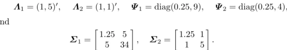
Λ1= (1,5)0, Λ2= (1,1)0, Ψ1= diag(0.25,9), Ψ2= diag(0.25,4),
and
Σ1=
1.25 5
5 34
, Σ2=
1.25 1
1 5
.
After drawing 100 points for each component, to check the robustness of our approach, we add some pointwise contaminationX3 to the data, in the form
of 11 points close to the point (4,50), as follows
X31∼4 + 0.03· N(0,1) X32∼50 + 0.03· N(0,1);
and 11 more points, denoted byX4, close to the point (6,-20), with
X41∼6 + 0.03· N(0,1) X42∼ −20 + 0.03· N(0,1).
Finally, we complement the data matrix, and the contamination, with stan-dard normally distributed random variablesXij ∼ N(0,1) forj = 3, . . . ,7.
In this way, we build a dataset where one factor is explaining the correlation among the 7 variables, in each component of the “regular” data, while no linear structure is embedded in the contamination.
0 2 4 6 8
−20
−10
0
10
20
30
40
50
0 2 4 6 8
−20
−10
0
10
20
30
40
50
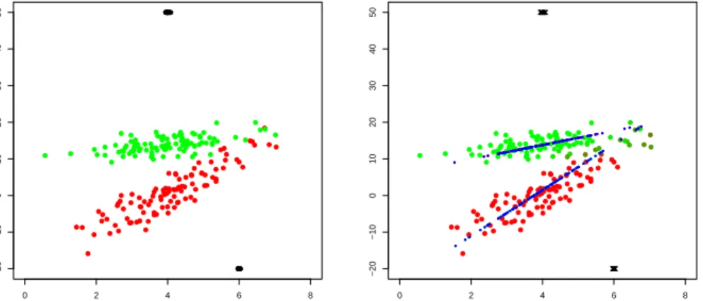
Fig. 1 Left panel: synthetic data (data drawn from X1 in green, fromX2 in red, and
contamination drawn fromX3andX4in black). Only the two first coordinates are plotted.
Right panel: Robust fuzzy classification of the synthetic data, with fuzzifierm= 1.1. Blue points are the factor scores of the 7-dimensional data in the estimated latent factor space. Black crosses (denoted by “×”) are trimmed units. The strength of the membership values is represented by the color usage: a mixture of red and green colors that can turn into brownish colors.
from the proposed robust estimation withα= 0.1. We see that the estimation is robust to the most dangerous outliers, like the pointwise contamination (although we have used the seven variables when applying the algorithm, only the first two variables are represented in the plots).
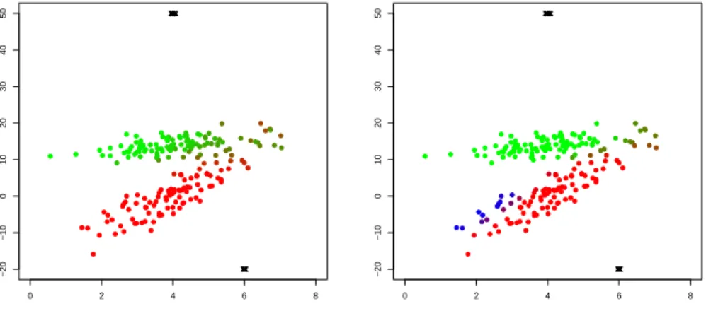
Noise matrices constraint: An important feature of our approach is rep-resented by the constrained estimation of the cluster scatters matrices. To show its effectiveness to discard spurious maximizers, we firstly perform a fuzzy clustering with c = 100, allowing some controlled variability within and between clusters eigenvalues, and successively we perform an almost un-constrained estimation, with c = 1010. Results for c = 1 have been shown
in Figure 1. In the right panel of Figure 2, we see that using c = 1010 and
searching for three clusters, we got a poor solution, with a few observations following a random pattern, clustered apart (in blue).
The fuzzifier parameterm: To observe the effect of the fuzzifier parameter
0 2 4 6 8
−20
−10
0
10
20
30
40
50
0 2 4 6 8
−20
−10
0
10
20
30
40
50
Fig. 2 Left panel: Fuzzy classification of the synthetic data, withc= 10 andG= 2. Right panel: Almost unconstrained fuzzy classification of the synthetic data, withc= 1010and
G= 3, generating a spurious solution. Blue points are belonging to a third component.
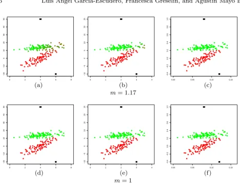
case, each observation is fully assigned to a cluster or trimmed off, as shown in Figure 3 (a). On the opposite side, we have all the non-trimmed observa-tions shared with approximately equal membership values for larger values ofm, likem= 1.2, as can be seen in Figure 3 (f). Intermediate values of m
yield perhaps more interesting membership values. By taking into account the updating step for the membership values in step 2.1.1 of the algorithm, it is important to see that “hard 0-1” clustering assignments can be done for observations clearly in the “cores” of the clusters. However, more fuzzy assignments (uig in the open (0,1) interval) may appear for observations
out-side these “cores”. This type of property was named as “hard contrast” in [39], to overcome a known shortcoming of fuzzy clustering. It is desirable, in-deed, that the cluster centers, which are weighted means of all objects, should not be influenced by observations that clearly do not belong to these clusters. An analogous effect would distort scatter matrices as well, computed inside the clustering algorithm. To avoid or at least highly reduce these unwanted effects, outlying objects should be discarded, clusters centers become crisp, whereas “doubtful” observations remain fuzzy assigned. To obtain such a so-lution, the choice of the value of m (also in relationship with an adequate scale) plays a key role.
0 2 4 6 8 −20 −10 0 10 20 30 40 50
0 2 4 6 8
−20 −10 0 10 20 30 40 50
0 2 4 6 8
−20 −10 0 10 20 30 40 50
(a) (b) (c)
0 2 4 6 8
−20 −10 0 10 20 30 40 50
0 2 4 6 8
−20 −10 0 10 20 30 40 50
0 2 4 6 8
−20 −10 0 10 20 30 40 50
(d) (e) (f)
Fig. 3 Effects of the value of the fuzzifier parametermon the cluster membership values (for panels (a), (b) and (c) we setm= 1,m= 1.1 andm= 1.13; while for panels (d), (e) and (f) we setm= 1.16,m= 1.17 andm= 1.2, respectively)
risk of incurring spurious solutions (as shown before). In this paragraph we want to discuss a second inherent issue, shared with other likelihood-based fuzzy clustering algorithms, as in [22], [46], [49] and [41]. Figure 4 shows in the first row panels the effect of the fuzzy clustering when all the variables in the artificial data are scaled by a constant factor, say divided by 2, in the second panel, and divided by 50 in the third one, consideringm= 1.17. There is an interplay between the scale and the fuzzifier parameter, in such a way that the scale of the variable leads to changes in the results whenm >1, while whenm= 1 (hard clustering) results are scale independent.
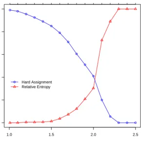
Hence, to suggest the user plausible values for the scale of the data and the fuzzifier parameter, in one only shot, we may base our analysis on some useful and well understandable quantities, like the percentage of hard assignment, and the relative entropy. The relative entropy is defined as
PG
g=1
Pn
i=1uigloguig
[n(1−α)] logG .
0 2 4 6 8 −20 −10 0 10 20 30 40 50
0 1 2 3 4
−10 −5 0 5 10 15 20 25
0.00 0.05 0.10 0.15
−0.4 −0.2 0.0 0.2 0.4 0.6 0.8 1.0
(a) (b) (c)
m= 1.17
0 2 4 6 8
−20 −10 0 10 20 30 40 50
0 1 2 3 4
−10 −5 0 5 10 15 20 25
0.00 0.05 0.10 0.15
−0.4 −0.2 0.0 0.2 0.4 0.6 0.8 1.0
(d) (e) (f)
m= 1
Fig. 4 In the upper panels, results of the robust fuzzy clustering withm= 1.17 obtained on the artificial data, when a change in scale is considered (from panel (a) to panel (b), all the variables have been scaled by a factor of 2, while in panel (c) by a factor of 50. In the lower panels, results of the hard clustering (withm= 1, same scaling as before, from left to right)
terms of hard assignment and relative entropy. Let us suppose that the user wants to obtain a clustering solution with 70% of observations crisply assigned and low relative entropy, say around 0.1. Inspecting the plot in Figure 5 we can derive guidelines for choosing a scale factor equal to 0.97 and a value
m = 1.7 for the fuzzifier parameter. By a scale factor we mean a number whichscales or multiply the values in a dataset.
1.0 1.5 2.0 2.5
0.0
0.2
0.4
0.6
0.8
1.0
m Hard Assignment Relative Entropy
0.67 0.7 0.73 0.77 0.81 0.86 0.91 0.97 1.03 1.11 1.2 1.3 1.43 1.58 1.76 2 scale
Fig. 5 Percentages of hard assignment (blue curve) and relative entropy (red curve) ob-tained when simultaneously changing the fuzzifier parameter and the scale.
the amount of noise in the data at hand, hence he can set the parameter
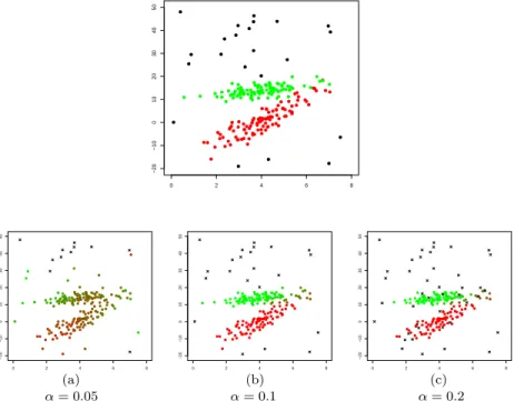
αaccordingly. If the contamination level is not known, we are interested in studying the effect of a value of αgreater/lower than needed, on the robust estimation. Figure 6 shows, in the upper panel, the data contaminated by noise, where the contamination is represented by the 22 black observations. In the three lower panels of the same Figure 6, we show the results of the robust estimation, when a lower than needed (α= 0.05, left panel), adequate (α = 0.1, central panel) and greater than needed trimming level (α = 0.2 right panel) have been adopted. We observe that the factor structure of the model is still recovered even for α= 0.2 where the trimming level is twice its correct value; while for α = 0.05 the estimation is poor (and for α= 0 it is spoiled out; results are not shown for sake of brevity). Based on our experience, we would suggest to start with a (high) conservative choice ofα
and then decrease it, on the light of a careful analysis of the plausibility of a few trimmed observations close to non trimmed ones.
To help the researcher to set a reasonable value for the trimming level, it is useful to recall that the quantitiesr(i)defined in (11) measure the evidence of
the belonging of observationxi to the estimated model. Data withr(i) lower
than r([nα)]) are identified as outlying observations and trimmed off. The
information conveyed by ther(i)values can be employed to give guidance on
0 2 4 6 8
−20
−10
0
10
20
30
40
50
0 2 4 6 8
−20
−10
0
10
20
30
40
50
0 2 4 6 8
−20
−10
0
10
20
30
40
50
0 2 4 6 8
−20
−10
0
10
20
30
40
50
(a) (b) (c)
α= 0.05 α= 0.1 α= 0.2
Fig. 6 Considering 22 noisy observations (in black) added to the original artificial dataset (upper panel), in the lower panels we show the results of the robust fuzzy clustering, with
m= 1.16, when a different trimming level is employed. The colors here represent the fuzzy membership values, whereas trimmed observations are denoted by black crosses.
(i/n, r(i))
n
i=1have been plotted, highlighting also theαvalue employed for
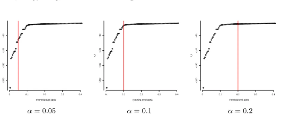
the estimation, with reference to the results shown in the three lower panels in Figure 6, respectively. The appropriate choice ofαcan be derived by finding an elbow in the plot, in other words a value α0 such that r(i) is steep for
i/n < α0 and the slope of the curve decreases for α > α0. For instance, in
the leftmost panel of Figure 7, we see that α = 0.05 is not a good choice, because the curve(i/n, r(i))
n
i=1is still quickly increasing aroundα= 0.05,
and the red line “cut” it too early, much before its elbow. On the opposite rightmost panel, we see that α = 0.2 would trim too much observations, and with some undesirable side effect, classifying points with almost equal contribution to the target function indifferently among the trimmed or among the non trimmed observations. The appropriate choice is suggested in the central panel, whereα= 0.1.
Trimming level alpha
r_i
0 0.1 0.2 0.3 0.4
−200
−150
−100
−50
Trimming level alpha
r_i
0 0.1 0.2 0.3 0.4
−200
−150
−100
−50
Trimming level alpha
r_i
0 0.1 0.2 0.3 0.4
−200
−150
−100
−50
α= 0.05 α= 0.1 α= 0.2
Fig. 7 Plots of the points
(i/n, r(i)) n
i=1, with reference to the robust fuzzy clustering
shown in the lower panels of Figure 6. The employed trimming levels are highlighted by the vertical lines.
trimmed likelihood curves”, once that a value for the parameterc has been set by the user (based on some previous knowledge that the user has on the data and/or on the type of clusters he is particularly interested in, depending on his/her final clustering purposes) and after incorporating the desired fuzzi-ness by the choice of the fuzzifier parameter m. These curves are graphical tools, obtained by plotting the target function for a range of values ofGand
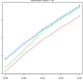
αthat can be inspected to derive a reasonable choice for these parameters. They were introduced in hard clustering problems in [20]). Figure 8 shows the classification trimmed likelihood curves obtained for the artificial dataset with added uniform noise, previously shown in the lower row panels in Figure 6. We monitor the maximum value obtained by the objective function (8), depending on a number of groups from 1 to 4, and a trimming level from 0 to 0.2. We see that, when reaching the trimming level α = 0.1, the results obtained for 2, 3 or 4 clusters almost virtually coincide. This means that with a lower trimming proportion, we would need a third or a fourth cluster to accommodate the noisy data. However, whenever the noisy observations have been identified and trimmed off, we are able to discover two main clusters in that artificial dataset.
5 An application to real data
fe-0.00 0.05 0.10 0.15 0.20
−2200
−2000
−1800
−1600
CTL−Curves
α
Objectiv
e Function V
alue
Restriction Factor = 50
4 4
4 4
4 4
4 4
4
3 3
3 3
3 3
3 3
3
2 2
2 2
2 2
2 2
2
1 1
1 1
1 1
1 1
1
Fig. 8 The classification trimmed likelihood curves for the artificial data, with added 0.1% noise, obtained withc= 50 andm= 1.1.
male athletes collected at the Australian Institute of Sport. It consists of 202 observations on the following 11 biometrical or hematological variables, apart from gender and sport: red cell count (RCC), white cell count (WCC), Hema-tocrit (Hc), Hemoglobin (Hg), plasma ferritin concentration (Fe), body mass index weight/height (BMI), sum of skin folds (SSF), body fat percentage (Bfat), lean body mass (LBM), height (in cm, Ht) and weight (in kg, Wt). The dataset is available within the sn package in R. We aim at studying the joint linear dependence among these biometrical and blood composition variables, through a fuzzy clustering method, to highlight atypical patterns and athletes’ features that would better require a fuzzy classification. We will exploit the conjecture that a strong correlation exists between the hematolog-ical and physhematolog-ical measurements. Therefore, a robust MFA may be estimated, assuming the existence of some underlying unknown factors (like nutritional status, hematological composition, body weight status indices, and so on) which jointly explain the observed measurements. We rely on previous work on this data in [21], where, based on a trimmed version of the Bayesian Information Criterion, the authors suggest to employ G = 2 clusters, and underlyingd= 6 factor dimension.
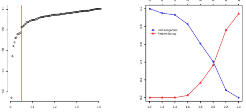
Aiming at selecting the value of the trimming level α, we employ the information conveyed by the sorted r(i) values. In the associated plot, we
the smallest contributions to the target function, when compared with the remaining data. This empirical approach, shown in the left panel of Figure 9, has suggested us the choice ofα= 0.05. Finally, to choose a scale factor and a value for the fuzzifier parameter m, we can base our decision on the desired percentage of hard assignments, jointly with the advisable relative entropy. The right panel of Figure 9 show us, once more, that the scale plays an important role in fuzzy clustering, due to its interplay with the fuzzifierm. As we are here dealing with multivariate data with disparate column scales (see Table 1), we need a different scale for each column. The value in the scale legend (upper horizontal legend) should be read as the multiple of the column standard deviation (or a robust variability measure) to be adopted for each variable in the dataset.
Trimming level alpha r(i)
0 0.1 0.2 0.3 0.4
−50
−40
−30
−20
−10
1.0 1.2 1.4 1.6 1.8 2.0 2.2 2.4
0.0
0.2
0.4
0.6
0.8
1.0
m Hard Assignment Relative Entropy
8 4 2.7 2 1.6 1.3 1.1 1 scale
Fig. 9 Plots for guiding the choice of the parameters when analyzing AIS data with fuzzy clustering. In the left panel we see how to choose the trimming levelα= 0.05. The right panel shows how to pick the fuzzifier parameterm and the scale, based on the desired percentage of hard assignment and the relative entropy.
Finally, we have chosen three different values of the fuzzifier, saym= 1.1,
m= 1.4 andm= 1.8 (on the scaled data) to show the effects of an increasing level of fuzziness (results in Figure 10).
identified both in the group of male ad female athletes: a firsthematological factor, with a very high loading on Hc, followed by RCC and Hg, and second factor, loading heavily on Ht, and in a lesser extent on Wt and LBM, that may be denoted as ageneral nutritional status. Hence observations that are consistently trimmed in the three plots are expected to have an unusual score on the factors.
The identification of outliers could have a very important role for the trainer or the physician that follow the team, to study a possible relation-ship among sport performances and exceptional values of some hematological and/or biometrical variables. Observing different membership levels, for this type of data, could also provide a particularly useful information. On the one side, athletes whose features are almost paradigmatic in their gender (or discipline) group are denoted by high levels of membership and can be easily identified. Like, for example, athlete in row 29, in the group of female, la-beled in the central plot of Figure 10, colored with full red (withu29,1= 0.999
and u29,2 = 0.001) has the features shown in first row of Table 1, that can
be interpreted as “paradigmatic”. Similar considerations hold for the ath-lete in row 188, in the group of male athath-letes, colored with full green (with
u188,1= 0.008 andu188,2= 0.993), whose measurements can be found in the
last row of Table 1, that can be considered as a prototype for male athletes. Conversely, athletes having unusual scores on the underlying factors, are denoted by low membership levels, and this could be a valuable information to be maintained up-to-date for team coachers, to assign a proper training regime, as well as for sport nutritionists to indicate an adequate diet. Such an example is athlete in row 70 where u70,1 = 0.511 and u70,2 = 0.489 or
athlete in row 130 withu130,1 = 0.469 andu130,2= 0.531. Table 1 reports
-in the second and third row - the observed variables for athletes that do not openly qualify for belonging to a group.
Table 1 Features for some athletes in the AIS dataset
row# gender sport RCC WCC Hc Hg Fe BMI SSF Bfat LBM Ht Wt 29 F Row 4.2 7.5 38.4 13.2 73 20.5 74.7 16.6 41.5 156.0 49.8 70 F Field 4.6 5.8 42.1 14.7 164 28.6 109.6 21.3 68.9 175.0 87.5 130 M B.Ball 4.5 5.9 44.4 15.6 97 20.7 41.5 7.2 73.0 195.3 78.9 188 M Row 4.8 9.3 43.0 14.7 150 25.1 60.2 10.0 78.0 186.0 86.8
At the end of this section, we would like to highlight the effectiveness of the proposed method, and compare it with other approaches in the litera-ture. The natural benchmarks to our proposal are the mixtures of Factor An-alyzers (MFA), and their robustification through trimming and constrained estimation in [21]. We may also want to compare with the fully parameter-ized Mixture of Gaussian (MG), in both robust and non-robust versions, as well as their fuzzy counterparts, to compare with previous work in [16]. Our first aim is to compare their clustering performances, reported in Table 2, when running the associated (trimmed and untrimmed) EM algorithm from 60 random initializations, with maximum number of iterations set to 30. To be more precise, the algorithm described in [21] is applied with α= 0 and
c = 1010 in the non-robust case for MFA and with α = 0.05 and c = 50 for robust MFA. We adopted the same choice of the parameters for the fully parameterized MG, estimated using thetclustpackage, for its fuzzy version described in [16], and for the proposed fuzzy MFA. To obtain Table 2, we have assigned even the trimmed observations, by resorting to the membership values that would have been obtained from the (robustly) estimated parame-ters and the proposed model. We can see that the proposed methodology has nice clustering performance, at least for the inspected values of the fuzzifier parameter m. Furthermore, we may appreciate the beneficial effect of us-ing trimmus-ing and also, for the AIS data, the advantage of combinus-ing robust methods with models that are able to capture the underlying latent struc-ture among variables. In other words, the model conveys how hematological factors and physical measurements play a slightly different role in male and in female athletes. Parsimony in model parameters has been pursued, too.
Table 2 Clustering performances of different models, in terms of number of misclassified units on the AIS dataset (different values of the fuzzifiermhave been considered for fuzzy clustering)
robust fuzzy MFA robust non-robust robust fuzzy MG robust non-robust
MFA MFA MG MG
m m
1.1 1.4 1.8 1.1 1.4 1.8
2 4 10 3 7 9 8 9 8 17
6 Concluding remarks
reduction. Second, it exploits the outlier tolerance advantages of procedures base on impartial trimming to provide a novel, soundly founded, nonheuris-tic, robust fuzzy clustering framework. Third, our proposal allows for soft as well as hard robust clustering, hence it encompasses both methodologies. Fourth, it enable the property of “hard contrast” of the solution: outlying ob-jects should be discarded, clusters centers become crisp, whereas “doubtful” observations remain fuzzy assigned.
This way, the proposed model yields a significant performance increase for the fuzzy clustering algorithm, as we experimentally demonstrate.
Comparing the fuzzy approach to classical model-based clustering via mix-tures, we would like to stress that in both methodologies we obtain a “degree of belonging” of thei-th observation to theg-th cluster. To contrast the two approaches, we remark that in the fuzzy approach we can control the level of fuzziness and/or a percentage of units to be crisply assigned to groups, as well as a relative entropy to be fulfilled by the solution, while in the mixture approach they arise as a byproduct of the estimated model. Based on our findings, we observed that small deviations from the model assumptions im-pair the performance of the fuzzy classifier only by a small amount, and that good efficiency is obtained on data without contamination.
With respect to robustness, that is our second qualifying point, roughly speaking, it is worth to recall that two main approaches can be found in the literature. The first, based on mixture modeling, aims at fitting the outliers in the model, e.g. by considering additional mixture components or by allowing heavy-tailed components. The second, based on trimming, just try to trim them off, without assuming any distribution for them. Hence, in comparison with fuzzy mixtures of Student’stfactor analyzers in [7], our proposal, being based on the constrained estimation of scatters and trimming off a proportion
αof the most outlying observations, provides good breakdown properties of the estimators (see [42] and [17]), in the sense of [27]. Yet, the complexity of the EM algorithm is considerably reduced, as it does not require the com-plicated estimation of the degree of freedom parameter, for which a closed solution in the EM algorithm is not available. Another interesting feature of our approach is that trimming, as a by-product, leads to the identification of outlying observations.
The effectivity of our proposal is also due to the parameters involved along the fuzzy robust estimation, like the noise matrices constraintc, the fuzzifier parameter m, the trimming levelα, the dimension of the underlying space
a way to identify athletes whose features are almost paradigmatic in their gender or discipline group, while athletes with low scores on the underlying factors, are a relevant information to be kept up-to-date for team coachers. Future research lines include developing more formal tools for helping the user to choose the several tuning parameters that this very flexible methodology requires.
References
1. A. Banerjee, R.N. Dav´e, Robust clustering, WIREs Data Mining Knowl Discov (2) (2012) 29–59.
2. J.C. Bezdek, Numerical taxonomy through fuzzy sets, J. Math. Biol. (1) (1974) 57–71. 3. C.M. Bishop, Latent variable models, in: Jordan, M.I. (Ed.), Learning in Graphical
Models, Kluwer, Dordrecht, 1998, pp. 371–403.
4. P.G. Bryant, Large-sample results for optimization-based clustering methods, J. Clas-sif. (8) (1991) 31–44.
5. R. Cattell, A note on correlation clusters and cluster search methods, Psychometrika 9(3) (1944) 169–184.
6. W. Chang, On Using Principal Components Before Separating a Mixture of Two Multivariate Normal Distributions, J. R. Stat. Soc. C-Appl. 32(3) (1983) 267–275. 7. S. Chatzis, T. Varvarigou, Factor analysis latent subspace modeling and robust fuzzy
clustering usingt-distributions, IEEE T. Fuzzy Syst. 17(3) (2009) 505–517.
8. R.D. Cook, S. Weisberg, An Introduction to Regression Graphics, John Wiley & Sons, New York, 1994.
9. J.A. Cuesta-Albertos, A. Gordaliza, C. Matr´an, Trimmed k-means: an attempt to robustify quantizers, Ann. Stat. 25(2)(1997) 553–576.
10. R.N. Dav´e, Characterization and detection of noise in clustering, Pattern Recogn. Lett. 12 (1991) 657–664.
11. R.N. Dav´e, R. Krishnapuram, Robust clustering methods: a unified view, IEEE T. Fuzzy Syst., 5 (1997) 270–293.
12. F. Dotto, A. Farcomeni, L.A. Garc´ıa-Escudero, A. Mayo-Iscar, A fuzzy approach to robust regression clustering, Adv. Data Anal. Classif. (2016) 1–20.
13. J.C. Dunn, A Fuzzy Relative of the ISODATA Process and Its Use in Detecting Compact Well-Separated Clusters, J. Cybernetics 3 (1973) 32–57.
14. A. Farcomeni, L. Greco, Robust Methods for Data Reduction, Chapman and Hall/CRC, 2015.
15. H. Fritz, L.A. Garc´ıa-Escudero, A. Mayo-Iscar, A fast algorithm for robust constrained clustering, Comput. Stat. Data An. 61(2013) 124–136.
16. H. Fritz, L.A. Garc´ıa-Escudero, A. Mayo-Iscar, Robust constrained fuzzy clustering, Inform. Sciences 245 (2013) 38–52.
17. M.T. Gallegos, G. Ritter, Trimming algorithms for clustering contaminated grouped data and their robustness, Adv. Data Anal. Classif., 3 (2009) 135–167.
18. L.A. Garc´ıa-Escudero, A. Gordaliza, C. Matr´an, A. Mayo-Iscar, A General Trimming Approach to Robust Cluster Analysis, Ann. Stat. 36 (3) (2008) 1324–1345.
19. L.A. Garc´ıa-Escudero, A. Gordaliza, C. Matr´an, A. Mayo-Iscar, A review of robust clustering methods, Adv. Data Anal. Classif. 4 (2010) 89–109.
20. L.A. Garc´ıa-Escudero, A. Gordaliza, C. Matr´an, A. Mayo-Iscar, Exploring the number of groups in robust model-based clustering, Stat. Comput. 21 (2011) 585–599. 21. L.A. Garc´ıa-Escudero, A. Gordaliza, F. Greselin, S. Ingrassia, A. Mayo-Iscar, The
22. I. Gath, A.B. Geva, Unsupervised optimal fuzzy clustering, IEEE T. Pattern Anal. 11(7) (1989) 773–780.
23. Z. Ghahramani, G.E. Hinton, The EM algorithm for factor analyzers, Technical Re-port No. CRG-TR-96-1, The University of Toronto, Toronto, 1996.
24. F. Greselin, S. Ingrassia, Maximum likelihood estimation in constrained parameter spaces for mixtures of factor analyzers, Stat. Comp. 25 (2015) 215–226.
25. E.E. Gustafson, W.C. Kessel, Fuzzy clustering with a fuzzy covariance matrix, in: Proceedings of the IEEE lnternational Conference on Fuzzy Systems, San Diego, 1979, pp. 761–766.
26. R. Hathaway, A constrained formulation of maximum-likelihood estimation for normal mixture distributions, Ann. Stat. 13(2) (1985) 795–800.
27. C. Hennig, Breakdown points for maximum likelihood estimators of location-scale mixtures, Ann. Stat. 32(4) (2004) 1313–1340.
28. G.E. Hinton, P. Dayan, M. Revow, Modeling the manifolds of images of handwritten digits, IEEE T. Neural Networ. 8 (1997) 65–73.
29. P.J. Huber, Robust Statistics, Wiley, New York, 1981.
30. S. Ingrassia, R. Rocci, Constrained monotone EM algorithms for finite mixture of multivariate Gaussians, Comput. Stat. Data An. 51 (2007) 5339–5351.
31. J. Kim, R. Krishnapuram, R. Dav´e, Application of the least trimmed squares tech-nique to prototype-based clustering, Pattern Recogn. Lett. 17 (1996) 633–641. 32. F. Klawonn, Noise clustering with a fixed fraction of noise, in: Applications and
Sci-ence in Soft Computing, Springer, Berlin-Heidelberg-New York, 2004, pp. 133–138. 33. R. Krishnapuram, J.M. Keller, A possibilistic approach to clustering, IEEE T. Fuzzy
Syst. 1 (1993) 98–110.
34. J. Leski, Towards a robust fuzzy clustering, Fuzzy Set. Syst. 37 (2003) 215–233. 35. J.B. MacQueen, Some Methods for classification and Analysis of Multivariate
Obser-vations, in: Proceedings of 5-th Berkeley Symposium on Mathematical Statistics and Probability, Berkeley, University of California Press, 1, 1967, pp. 281–297 .
36. G.J. McLachlan., D. Peel, Finite Mixture Models, John Wiley & Sons, New York, 2000.
37. S. Miyamoto, M. Mukaidono, Fuzzyc-means as a regularization and maximum entropy approach, in: Proceedings of the 7th International Fuzzy Systems Association World Congress, IFSA’97, 2, 1997, pp. 86–92.
38. G. Ritter, Robust Cluster Analysis and Variable Selection, Chapman & Hall/CRC Monographs on Statistics & Applied Probability, 2015.
39. P.J. Rousseeuw, E. Trauwaert, L. Kaufman, Fuzzy clustering with high contrast, J. Comput. Appl. Math. 64 (1995) 81–90.
40. P.J. Rousseeuw, K. Van Driessen, A fast algorithm for the minimum covariance de-terminant estimator, Technometrics 41 (1999) 212–223.
41. P.J. Rousseeuw, L. Kauffman, E. Trauwaert, Fuzzy clustering using scatter matrices, Comput. Stat. Data An. 23 (1996) 135–151.
42. C. Ruwet, L.A. Garc´ıa-Escudero, A. Gordaliza, A. Mayo-Iscar, On the breakdown behavior of the TCLUST clustering procedure, Test, 22 (3) (2013) 466–487. 43. M.J. Symons, Clustering criteria and multivariate normal mixtures, Biometrics 37
(1981) 35–43.
44. M.E. Tipping, C.M. Bishop, Mixtures of probabilistic principal component analysers, Technical Report No. NCRG=97=003, Neural Computing Research Group, Aston University, Birmingham, 1997.
45. M.E. Tipping, C.M. Bishop, Mixtures of probabilistic principal component analysers, Neural Comput. 11 (1999) 443–482.
46. E. Trauwaert, L. Kaufman, P. Rousseeuw, Fuzzy clustering algorithms based on the maximum likelihood principle, Fuzzy Set. Syst. 42(2) (1991) 213–227.
48. K.L. Wu, M.S. Yang, Alternativec-means clustering algorithms, Pattern Recogn. 35 (2002) 2267–2278.
49. M.S. Yang, On a class of fuzzy classification maximum likelihood procedures, Fuzzy Set. Syst. 57 (1993) 365–375.
FUZZY SET SYST
−2 −1 0 1 2 3 4
−1
0
1
2
3
4
BMI
SSF
11
68
75
93
99
133
160 163
166
178
−2 −1 0 1 2 3 4
−1
0
1
2
3
4
BMI
SSF
29−
70−
118−
130−
−2 −1 0 1 2 3 4
−1
0
1
2
3
4
BMI
SSF