arXiv:1503.06302v1 [stat.ME] 21 Mar 2015
Robust estimation for mixtures of Gaussian factor analyzers,
based on trimming and constraints
L.A. Garc´ıa-Escuderoa, A. Gordalizaa, F. Greselinb, S. Ingrassiac, A. Mayo-Iscara
aDepartment of Statistics and Operations Research and IMUVA, University of Valladolid, Valladolid, Spain
bDepartment of Statistics and Quantitative Methods, Milano-Bicocca University, Milan, Italy
cDepartment of Economics and Business, University of Catania, Catania, Italy
Abstract. Mixtures of Gaussian factors are powerful tools for modeling an
unob-served heterogeneous population, offering - at the same time - dimension
reduc-tion and model-based clustering. Unfortunately, the high prevalence of spurious
solutions and the disturbing effects of outlying observations, along maximum
like-lihood estimation, open serious issues. In this paper we consider restrictions for
the component covariances, to avoid spurious solutions, and trimming, to provide
robustness against violations of normality assumptions of the underlying latent
fac-tors. A detailed AECM algorithm for this new approach is presented. Simulation
results and an application to the AIS dataset show the aim and effectiveness of the
proposed methodology.
Keywords: Constrained estimation; Factor Analyzers Modeling; Mixture Models;
Model-Based Clustering; Trimming; Robust estimation.
Contents
1 Introduction and motivation 2
2 Gaussian Mixtures of Factor Analyzers 4
3 Trimmed Mixtures of Factor Analyzers 5
3.1 Problem statement . . . 5
3.2 Algorithm . . . 6
4 Numerical studies 12
4.1 Artificial data . . . 12
4.1.1 Properties of the estimators for the mixture parameters . . . 15
5 Concluding remarks 26
1
Introduction and motivation
Factor analysis is an effective method of summarizing the variability between a number of
cor-related features, through a much smaller number of unobservable, hence named latent, factors.
It originated from the consideration that, in many phenomena, several observed variables could
be explained by a few unobserved ones. Under this approach, each single observed variable
(among thepones) is assumed to be a linear combination ofdunderlying common factors with
an accompanying error term to account for that part of variability that is unique to it (not in
common with other variables). Ideally, d should be substantially smaller than p, to achieve
parsimony.
Clearly, the effectiveness of this method is limited by its global linearity, as it happens
for principal components analysis. Hence, Ghahramani and Hilton (1997), Tipping and Bishop
(1999) and McLachlan and Peel (2000a) solidly widened the applicability of these approaches
by combining local models of Gaussian factors in the form of finite mixtures. The idea is to
employ latent variables to perform dimensional reduction in each component, thus providing
a statistical method which concurrently performs clustering and, within each cluster, local
di-mensionality reduction.
In the literature, error and factors are routinely assumed to have a Gaussian distribution
be-cause of their mathematical and computational tractability: however statistical methods which
ignore departure from normality may cause biased or misleading inference. Moreover, it is
well known that maximum likelihood estimation for mixtures often leads to ill-posed problems
because of the unboundedness of the objective function to be maximized, which favors the
appearance of non-interesting local maximizers and degenerate or spurious solutions.
The lack of robustness in mixture fitting arises whenever the sample contains a certain
pro-portion of data that does not follow the underlying population model. Spurious solutions can
even appear when ML estimation is applied to artificial data drawn from a given finite mixture
model, i.e. without adding any kind of contamination. Hence, robustified estimation is needed.
Many contributions in this sense can be found in the literature: from Mclust model with a noise
component in Fraley and Raftery (1998), mixtures of t-distributions in McLachlan and Peel
(1998), the trimmed likelihood mixture fitting method in Neykov et al. (2007), the trimmed ML
ML estimator introduced in Coretto and Hennig (2011), among many others. Some important
applications in fields like computer vision, pattern recognition, analysis of microarray gene
ex-pression data, or tomography (see, for example, Stewart (1999), Campbell et al. (1997), Bickel
(2003) and Maitra (2001), respectively) suggest that more attention should be paid to
robust-ness, because noise in the data sets may be frequent in all these fields of application.
Different types of constraints have been traditionally applied in Gaussian mixtures of factor
analyzers, for instance, some authors propose to take a common (diagonal) error matrix (as
for the Mixtures of Common Factor Analyzers, denoted by MCFA, in Baek et al., 2010) or
to impose an isotropic error matrix Bishop and Tipping, 1998. This strategy has proven to
be effective in many cases, at the expenses of stronger distributional restrictions on the data.
In McNicholas and Murphy, 2008, when analyzing parsimonious mixtures of Gaussians factor
analyzers models, they realized that equal determinant restrictions give more stable results. For
avoiding singularities and spurious solutions, under milder conditions, Greselin and Ingrassia
(2013) recently proposed to maximize the likelihood by constraining the eigenvalues of the
covariance matrices, following previous work of Ingrassia (2004) and going back to Hathaway
(1985). Furthermore, McLachlan and Bean (2005), Baek and McLachlan (2011), Steane et al.
(2012) and Lin et al. (2014) have considered the use of mixtures oft-analyzers in an attempt
to make the model less sensitive to outliers, but they, too, are not robust against very extreme
outliers (Hennig, 2004); while Fokou´e and Titterington (2003) proposed a Bayesian approach.
The purpose of the present work is to introduce an estimating procedure for mixture of
Gaussian factors analyzers that can resist the effect of outliers and avoid spurious local
maxi-mizers. The proposed constraints can be also used to take into account prior information about
the scatter parameters.
Trimming has been shown to be a simple, powerful, flexible and computationally feasible
way to provide robustness in many different statistical frameworks. The basic idea behind
trimming here is the removal of a little proportion α of observations whose values would be
the more unlikely to occur if the fitted model was true. In this way, trimming avoids that a
small fraction of outlying observations could exert a harmful effect on the estimation of the
parameters of the fitted model.
Incorporating constraints in the mixture fitting estimation method moves the mathematical
problem in a well-posed setting and hence minimizes the risk of incurring spurious solutions.
Moreover, a correct statement of the problem allows to study the properties of the EM
estimators, such as the existence and consistency results, as in Garc´ıa-Escudero et al. (2008)
and Gallegos and Ritter (2009).
We have organized the rest of the paper as follows. In Section 2 we introduce notation
and summarize main ideas about Gaussian Mixtures of Factor Analyzers (in the foremost,
de-noted by MFA). Then, in Section 3 we introduce the trimmed likelihood for MFA and we
pro-vide fairly extensive notes concerning the EM algorithm, with incorporated trimming and
con-strained estimation. In Section 4 we discuss the performance of our procedure, on the ground
of some numerical results obtained from simulated and real data. In particular, we compare the
bias and MSE of robustly estimated model parameters for different cases of data contamination,
by Monte Carlo experiments. The application to the Australian Institute of Sports dataset shows
how classification and factor analysis can be developed using the new model. Section 5 contains
concluding notes and provides ideas for further research.
2
Gaussian Mixtures of Factor Analyzers
The density of the p-dimensional random variable X of interest is modeled as a mixture of
Gmultivariate normal densities in some unknown proportions π1, . . . πG, whenever each data
point is taken to be a realization of the following density function,
f(x;θ) =
G
X
g=1
πgφp(x;µg,Σg) (2.1)
whereφp(x;µ,Σ)denotes thep-variate normal density function with mean vectorµand
covari-ance matrixΣ. Here the vectorθ=θGM(p, G)of unknown parameters consists of the(G−1)
mixing proportionsπg, theGpelements of the component meansµg, and the12Gp(p+1)distinct
elements of the component-covariance matricesΣg. MFA postulates a finite mixture of linear
sub-models for the distribution of the full observation vectorX, given the (unobservable)
fac-torsU. That is, MFA provides local dimensionality reduction by assuming that the distribution
of the observationXican be given as
Xi =µ
g+ΛgUig+eig with probability πg(g = 1, . . . , G) fori= 1, . . . , n, (2.2)
whereΛgis ap×dmatrix of factor loadings, the factorsU1g, . . . ,UngareN(0,Id)distributed
independently of the errorseig. The latter are independentlyN(0,Ψg)distributed, andΨg is
ap×pdiagonal matrix(g = 1, . . . , G). The diagonality ofΨg is one of the key assumptions
variablesUig model correlations between the elements ofXi, while the errorseig account for
independent noise forXi. We suppose thatd < p, which means thatdunobservable factors are
jointly explaining the p observable features of the statistical units. Under these assumptions,
the mixture of factor analyzers model is given by (2.1), where theg-th component-covariance
matrixΣg has the form
Σg =ΛgΛ′
g+Ψg (g = 1, . . . , G). (2.3)
The parameter vectorθ=θM F A(p, d, G)now consists of the elements of the component means
µg, theΛg, and theΨg, along with the mixing proportionsπg (g = 1, . . . , G−1), on putting
πG = 1−PGi=1−1πg.
3
Trimmed Mixtures of Factor Analyzers
In this section we present the trimmed (Gaussian) mixtures of factor analyzers model (trimmed
MFA) and we propose a feasible algorithm for its implementation.
3.1
Problem statement
We will fit a mixture of Gaussian factor components to a given datasetx={x1,x2, . . . ,xn}in
Rpby maximizing a trimmed mixture log-likelihood (see Neykov et al. 2007, Gallegos and Ritter 2009 and Garc´ıa-Escudero et al. 2014) defined as:
Ltrim =
n
X
i=1
z(xi) log " G
X
g=1
φp(xi;µg,ΛgΛ′g+Ψg)πg
#
(3.1)
wherez(·)is a 0-1 trimming indicator function that tell us whether observationxi is trimmed
off:z(xi)=0, or not:z(xi)=1 andΣg =ΛgΛ′
g +Ψg as in (2.3). A fixed fractionαof
observa-tions can be unassigned by settingPn
i=1z(xi) = [n(1−α)]. Hence the parameterαdenotes the
trimming level. As usual, x1, . . . ,xn are the realized values of n independent and identically
distributed random vectorsX1, . . . ,Xn with common density given in (2.1), with
component-covariance matricesΣgas in (2.3) forg = 1, . . . , G. The component label vectorsz1, . . . ,znare
taken to be the realized values of the random vectorsZ1, . . . ,Zn, where, for independent feature
data, it is appropriate to assume that they are (unconditionally) multinomially distributed. i.e.
Moreover, to avoid the unboundedness ofLtrim, we introduce a constrained maximization
of (3.1). In more detail, with reference to the diagonal elements {ψg,k}k=1,...,p of the noise
matricesΨg forg = 1, . . . , Gwe require that
ψg1,k ≤cnoise ψg2,h for every1≤k =6 h≤pand1≤g1 6=g2 ≤G (3.2)
The constant cnoise is finite and such that cnoise ≥ 1, to avoid the |Σg| → 0 case. This
constraint can be seen as an adaptation to MFA of those introduced in Ingrassia and Rocci
(2007), Garc´ıa-Escudero et al. (2008) and it is similar to the mild restrictions implemented for
MFA in Greselin and Ingrassia (2013). They all go back to the seminal paper of Hathaway
(1985). We will look for the ML estimators ofΨg under the given constraints, and this position
set the maximization problem as a well-defined one, and at the same time discard singularities
and reduce spurious solutions.
If {λk(A)}k=1,...,p denote the set of eigenvalues of the p × p matrix A, a second set of
constraints apply on the product of the loading matricesΛgΛ′
g by requiring that
λk(Λg1Λ
′
g1)≤cload λh(Λg2Λ
′
g2)for every1≤k6=h≤dand1≤g1 6=g2 ≤G. (3.3)
withcload such that1 ≤ cload < +∞. Theseλk(ΛgΛ′g)values control the different scatters in
the reduced subspaces. In fact, these type of constraints are not needed to avoid singularities in
the target function but they could be useful to achieve more sensible solutions.
In the foremost, we will denote byΘc the constrained parameter space forθ={πg, µg,Ψg,
Λg;g = 1, . . . , G}under the requirements (3.2) and (3.3).
3.2
Algorithm
The maximization of Ltrim in (3.1) for θ ∈ Θc is not an easy task, obviously. We will give
a feasible algorithm obtained by combining the Alternating Expectation-Conditional
Maxi-mization algorithm (AECM) for MFA with that (with trimming and constraints) introduced
in Garc´ıa-Escudero et al. (2014) (see, also, Fritz et al., 2013).
The AECM is an extension of the EM, suggested by the factor structure of the model, that
uses different specifications of missing data at each stage. The idea is to partition the vector of
parametersθ = (θ′
1,θ′2)′ in such a way thatLtrim is easy to be maximized forθ1givenθ2and
viceversa, replacing the M-step by a number of computationally simpler conditional
maximiza-tion (CM) steps. In more detail, in the first cycle we set θ1 ={πg,µg;g = 1, . . . , G}and the
missing data are the unobserved group labelsZ = (z′
θ2 ={Λg,Ψg;g = 1, . . . , G}and the missing data are the group labelsZand the unobserved
latent factors U = (U11, . . . ,UnG). Hence, the application of the AECM algorithm consists
of two cycles, and there is one E-step and one CM-step alternatively considering θ1 and θ2
in each cycle. Before describing the algorithm, we remark that the unobserved group labels
Zare considered missing data in both cycles. Therefore, during thel-th iteration, we shall
de-note byzig(l+1/2)andzig(l+1)the conditional expectations at the first and second cycle, respectively.
The algorithm has to be run multiple times on the same dataset, with different starting
values, to prevent the attainment of a local, rather than global, maximum log-likelihood. In
each run it executes the following steps:
1 Initialization:
Each iteration begins by selecting initial values for θ(0) where θ(0) = (π(0)
g , µ(0)g ,Λ(0)g ,
Ψ(0)
g ;g = 1, . . . , G). Inspired from results obtained in a series of extensive test
experi-ments about initialization strategies (see Maitra, 2009), and aiming to allow the algorithm
to visit the entire parameter space, we randomly selectp+ 1units (without replacement)
for groupg from the observed data x = {xi}i=1,...,n. In this way we obtain a
subsam-pleXg that we arrange in a (p+ 1)×pmatrix, and its sample mean will be the initial
µ(0)g .Additionally, based on thesep+1observations, we developed a new ad hoc approach
for providing an initialization procedure for Ψ(0)
g and Λ(0)g , to deal with the possible
ex-istence of gross outlying observations among the subsamples, which could inflate
dis-proportionally some of their eigenvalues. The rationale under our procedure is, as usual,
to fill in randomly the missing information in the complete model through random
sub-samples and, then, to estimate the other parameters. The missing information here are
the factors u1, . . . ,un, which, under the assumptions for the model, are independently
N(0,Id)distributed. We consider model (2.2) in groupg as a regression ofXi with
in-terceptµg, regression coefficients given byΛg, where the explanatory variables are the
latent factorsUig, and with regression errorseig. Hence we drawp+ 1random
observa-tions from thed-variate standard Gaussian to fill a (p+ 1)×dmatrixUg. Then we set
Λ(0)
g = (U′gUg)−1Ug′Xgc whereXgc is obtained by centering the columns of theXg
ma-trix. To provide a restricted random generation ofΨg, we compute the(p+ 1)×pmatrix
εg =xgc−Λ(0)g Ug, and we set the diagonal elements ofΨ(0)g equal to the variances of the
Λ(0)
g andΨ(0)g do not satisfy the required constraints (3.2) and (3.3), then the constrained
maximizations described in step 2.4 must be applied. Finally, weightsπ(0)1 , ..., π(0)G in the
interval(0,1)and summing up to 1 are randomly chosen.
2 Trimmed AECM steps:
The following steps 2.1–2.4. are alternatively executed until convergence (i.e. ||z(l+1)−
z(l)|| < ǫ) for a small constantǫ > 0or until reaching a maximum number of iterations
MaxIter. The implementation of trimming is related to the “concentration” steps applied
in high-breakdown robust methods (Rousseeuw and Van Driessen, 1999). Trimming is
performed along the E-steps, while constraints are enforced during the second cycle CM
step.
2.1 First cycle. E-step:
Here θ1 = {πg,µg;g = 1, . . . , G}and the missing data are the unobserved group
labels z = (z′
1, . . . ,z′n). The E-step on the first cycle on the (l + 1)-th iteration
requires the calculation of
Q1
θ1;θ(l)
=Eθ(l)
Ltrim(θ1)|x
,
which is the expected trimmed complete-data log-likelihood given the data xand
using the current estimateθ(l) forθ. In practice it requires calculatingE
θ(l)[Zig|x] and usual computations show that this step is achieved by replacing each zig by its
current conditional expectation given the observed dataxi, that is we replacezig by
τig(l+1/2), where the latter is evaluated as follows. Let us define
Dg x;θ(l)
=φp
x;µ(l)
g ,Λ(gl)
Λ(l)
g
′
+Ψ(l)
g
π(gl)
and
Di =D xi;θ(l)
=
G
X
g=1
Dg xi;θ(l)
, fori= 1, ..., n.
After sorting these n values, the notationD(1) ≤ .... ≤ D(n) is adopted. Let us
consider the subset of indicesI ⊂ {1,2, ..., n}defined as
I =
To update the parameters, only the observations with indices inI will be taken into
account. In other words, we are tentatively discarding the proportionαof
observa-tions with the smallestD(i)values.
Then, set
τig(l+1/2) =
Dg(xi;θ(l))
D(xi;θ(l)) fori∈I
0 fori /∈I.
Note that, for the observations with indices inI,τig(l+1/2) are the “posterior
probabil-ities” often considered in standard EM algorithms applied when fitting MFAs. But,
unlike the standard EM algorithms, the τig(l+1/2) (and consequently the zig) for the
discarded observations are set to 0.
2.2 First cycle. CM-step: This first CM step requires the maximization of Q1(θ1;θ(l))
overθ, withθ2 held fixed atθ(2l). We getθ (l+1)
1 by updatingπgandµg as follows
π(l+1)
g =
Pn
i=1τ (l+1/2)
ig
[n(1−α)]
and
µ(gl+1) = Pn
i=1τ (l+1/2)
ig xi
n(gl+1/2)
wheren(gl+1/2) =Pni=1τig(l+1/2), forg = 1, . . . , G. According to notation in McLachlan and Peel
(2000b), we setθ(l+1/2) =θ1(l+1),θ(2l)′.
2.3 Second cycle. E- step:
Here we consider θ2 = {(Λg, Ψg), g = 1, . . . , G}, where the missing data are
the unobserved group labels Z and the latent factors U. Therefore, the trimmed
complete-data log-likelihood in this second cycle may be written as
Ltrim:2(θ2) =
n
X
i=1
z(xi) log
G
X
g=1
φp xi;µg(l+1) −Λguig,Ψg
φd(uig; 0,Id)πg(l+1)
.
The E-step on the second cycle on the l-th iteration requires the calculation of the
conditional expectation of Ltrim:2, given the observed dataxand using the current
estimateθ(l+1/2)forθ, i.e.
Q2
θ2;θ(l+1/2)
=Eθ(l+1/2)
Ltrim:2(θ2)|x
In addition to updating the posterior probabilities E
θ(l+1/2)[Zig|x] by performing a concentration step and replacing eachzigby the new valuesz(igl+1) =τ
(l+1)
ig (and
con-sequently n(gl+1) = Pni=1τig(l+1), for g = 1, . . . , G, as previously done in step 2.1),
this leads to evaluate the following conditional expectations: E
θ(l+1/2)[ZigUig|x] andE
θ(l+1/2)[ZigUigU′ig|x]. Recalling that the conditional distribution ofUig given
xi is
Uig|xi ∼ N γ
g(xi−µg),Iq−γgΛg
fori= 1, . . . , nandg = 1, . . . , Gwith
γg =Λ′
g(ΛgΛ′g +Ψg)−1,
we obtain
Eθ(l+1/2)[ZigUig|xi] =zig(l+1)γ(gl) xi−µ(gl+1)
Eθ(l+1/2)[ZigUigU′ig|xi] =zig(l+1)
γ(gl) xi−µ(l+1)
g
xi−µ(l+1)
g
′
γ(gl)′+Iq−γ(l)
g Λ(gl)
=zig(l+1)Ξ(l)
ig,
where we set
γ(gl) =Λ(l)
g
′ Λ(l)
g Λ(gl)
′
+Ψ(l)
g
−1
Ξ(l)
ig =Iq−γ(gl)Λg(l)+γg(l+1) xi−µ(gl+1)
xi −µ(l+1)
g
′
γ(gl)′.
2.4 Second cycle. CM-step for constrained estimation ofΛgandΨg :
Here our aim is to maximizeQ2
θ2;θ(l)
overθ, withθ1held fixed atθ(1l+1). After
some matrix algebra, this yields the updated ML-estimates
Λg =S(gl+1)γ(l)′g[Ξ(gl)]−1
Ψg =diagnS(l+1)
g −Λ(gl+1)γg(l)S(gl+1)
o
where we denote byS(gl+1)the sample scatter matrix in groupg, forg = 1, . . . , G
S(l+1)
g = (1/n(gl+1)) n
X
i=1
zig(l+1) xi−µ(l+1)
g
xi−µ(l+1)
g
′
.
Along the iterations, due to the updates, it may happen that the Λg matrices do
the ΛgΛ′
g matrices do not satisfy the required constraint (3.3), we obtain the ML
solution in Θc by projecting the unconstrained optimum intoΘc. To this aim, the
singular-value decomposition ofΛgΛ′
g =L′gEgLg is considered, withLg being an
orthogonal matrix and Eg = diag(eg1, eg2, ..., egd) a diagonal matrix (notice that
some of these egk may be equal to 0 if ΛgΛ′g is not full rank). Truncated singular
values are then defined as
[egk]m = min(cload·m,(max(egk, m))), for k = 1, . . . , dandg = 1, . . . , G,
and m being some threshold value. The loading matrices are finally updated as
Λ(l+1)
g such thatΛ(gl+1)
Λ(l+1)
g
′ =L′
gE∗gLg with
E∗
g =diag [eg1]mopt,[eg2]mopt, ...,[egd]mopt
andmopt minimizing the real valued function
fload(m) =
G
X
g=1
π(l+1)
g d
X
k=1
log ([egk]m) +
egk
[egk]m
. (3.5)
It may be mentioned here, in passing, that Proposition 3.2 in Fritz et al. (2013)
shows thatmoptcan be obtained by evaluating2dG+1times the real valued function
fload(m)in (3.5).
Given theΛ(l+1)
g , we obtain the matrices
Ψg =diagnS(l+1)
g −Λ(gl+1)γg(l)S(gl+1)
o
which may not necessarily satisfy the required constraint (3.2). In this case, we set
[ψg,k]m = min(cnoise·m, max(ψg,l, m)), for k = 1, . . . , d;g = 1, . . . , G,
and fix the optimal threshold value mopt by minimizing the following real valued
function
fnoise(m)7→ G
X
g=1
πg(l+1)
p
X
k=1
log ([ψg,k]m) +
ψg,k
[ψg,k]m
. (3.6)
As before, in Fritz et al. (2013) it is shown thatmopt can be obtained in a straightful
way by evaluating2pG+ 1timesfnoise(m)in (3.6). Thus,Ψ(gl+1)is finally updated
as
Ψ(l+1)
g =diag([ψg,1]mopt, ...,[ψg,p]mopt).
It is worth to remark that the given constrained estimation provides, at each step,
the parametersΨg and Λg maximizing the likelihood in the constrained parameter
3 Evaluate target function: After applying the trimmed and constrained EM steps, and
setting z(xi) = 0 if i ∈ I and z(xi) = 1 if i /∈ I, the associated value of the target
function (3.1) is evaluated. If convergence has not been achieved before reaching the
maximum number of iterationsMaxIter, results are discarded.
The set of parameters yielding the highest value of the target function (among the multiple runs)
and the associated trimmed indicator functionzare returned as the final output of the algorithm.
In the framework of model-based clustering, each unit is assigned to one group, based on the
maximum a posteriori probability. Notice, in passing, that we do not need a high number of
initializations neither a high value forMaxIter, as we will see in Section 4.
4
Numerical studies
In this section we present numerical studies, based on simulated and real data, to show the
performance of the constrained and trimmed AECM algorithm with respect to unconstrained
and/or untrimmed approaches.
4.1
Artificial data
We consider here the following mixture of G components of d-variate normal distributions.
To perform the estimation, we consider 10 different random initial clusterings to initialize the
algorithm at each run, as described in the previous section, and we retain the best solution. The
needed routines have been written inR-code (R Team, 2013), and are available from the authors
upon request.
MIXTURE: G= 3,d = 6, q= 2,N = 150.
The sample has been generated with weightsπ = (0.3,0.4,0.3)′ according to the following
parameters:
µ1= (0,0,0,0,0,0)′ Ψ1=diag(0.1,0.1,0.1,0.1,0.1,0.1)
µ2= (5,5,5,5,5,5)′ Ψ2=diag(0.4,0.4,0.4,0.4,0.4,0.4)
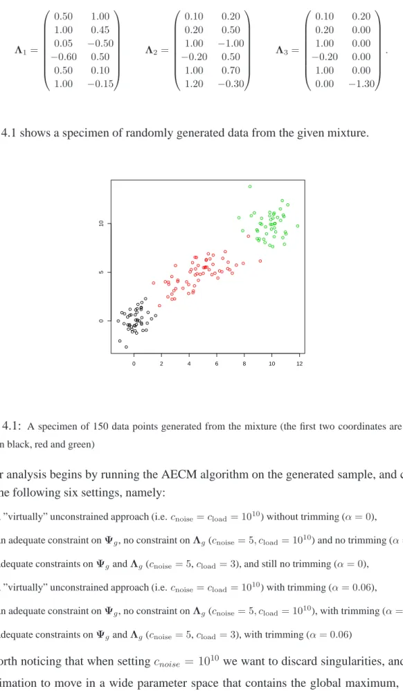
Λ1=
0.50 1.00 1.00 0.45 0.05 −0.50
−0.60 0.50
0.50 0.10 1.00 −0.15
Λ2=
0.10 0.20 0.20 0.50 1.00 −1.00
−0.20 0.50
1.00 0.70 1.20 −0.30
Λ3=
0.10 0.20 0.20 0.00 1.00 0.00
−0.20 0.00
1.00 0.00 0.00 −1.30
.
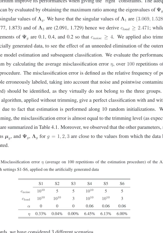
Figure 4.1 shows a specimen of randomly generated data from the given mixture.
0 2 4 6 8 10 12
0
5
10
Figure 4.1: A specimen of 150 data points generated from the mixture (the first two coordinates are plotted,
groups in black, red and green)
Our analysis begins by running the AECM algorithm on the generated sample, and consid-ering the following six settings, namely:
S1. a ”virtually” unconstrained approach (i.e.cnoise=cload= 1010) without trimming (α= 0),
S2. an adequate constraint onΨg, no constraint onΛg(cnoise= 5, cload= 1010) and no trimming (α= 0), S3. adequate constraints onΨgandΛg(cnoise= 5,cload= 3), and still no trimming (α= 0),
S4. a ”virtually” unconstrained approach (i.e.cnoise=cload= 10 10
) with trimming (α= 0.06), S5. an adequate constraint onΨg, no constraint onΛg(cnoise= 5, cload= 10
10
), with trimming (α= 0.06), S6. adequate constraints onΨgandΛg(cnoise= 5,cload= 3), with trimming (α= 0.06)
It is worth noticing that when settingcnoise = 1010 we want to discard singularities, and allow
the estimation to move in a wide parameter space that contains the global maximum, among
that the algorithm improve its performances when giving the ”right” constraints. The adequate
constraints can by evaluated by obtaining the maximum ratio among the eigenvalues ofΨgand
among the singular values ofΛg. We have that the singular values ofΛ1 are(3.069,1.528), of
Λ2 are (3.777, 1.873) and ofΛ3 are (2.091, 1.729) hence we derivecload ≥ 2.471; while the
diagonal elements of Ψg are 0.1, 0.4, and 0.2 so that cnoise ≥ 4. We applied also trimming
to the artificially generated data, to see the effect of an unneeded elimination of the outermost
points in the model estimation and subsequent classification. We evaluate the performance of
the algorithm by calculating the average misclassification error η, over 100 repetitions of the
estimation procedure. The misclassification error is defined as the relative frequency of points
of the sample erroneously labeled, taking into account that noise and pointwise contamination
(when added) should be identified, as they virtually do not belong to the three groups. We
see that the algorithm, applied without trimming, give a perfect classification with and without
constraints, due to fact that estimation is performed along 10 random initializations. While
adding trimming, the misclassification error is almost equal to the trimming level (as expected).
The results are summarized in Table 4.1. Moreover, we observed that the other parameters, such
as the means µg, andΨg, Λg for g = 1,2,3are close to the values from which the data have
been generated.
Table 4.1: Misclassification error η (average on 100 repetitions of the estimation procedure) of the AECM algorithm with settings S1-S6, applied on the artificially generated data
S1 S2 S3 S4 S5 S6
cnoise 1010 5 5 1010 5 5
cload 1010 1010 3 1010 1010 3
α 0 0 0 0.06 0.06 0.06
η 0.33% 0.04% 0.00% 6.45% 6.13% 6.00%
Afterwards, we have considered 3 different scenarios.
D+N: 10 points of uniform noise have been added around the data,
D+PC: 10 points of pointwise contamination have been added outside the range of the data,
D+N+PC: both the uniform noise and the pointwise contamination have been added to the data.
We applied the algorithm to the different datasets in the six previous settings S1-S6 (i.e. with/without
constraints and trimming) and we calculated the misclassification error. Results in the first row
of Table 4.2 show that trimming is very effective to identify and discard noise in the data, and
(re-ported in the second row of Table 4.2) shows that we need trimming and constraints to achieve
a very good behavior of the algorithm. Noise and pointwise contamination could cause very
messy estimation, as it is seen in the first three columns of the Table, where we only rely/do
not rely on constraints. Further, we observe that trimming is a good strategy when dealing with
uniform noise, but it is not able to resist pointwise contamination. If we want to be protected
against all type of data contamination we do need both the use of constrained estimation and
trimming.
Table 4.2: Misclassification error η (average on 100 repetitions of the estimation procedure) of the AECM algorithm with settings S1-S6, applied on different data sets
S1 S2 S3 S4 S5 S6
cnoise 1010 5 5 1010 5 5
cload 1010 1010 3 1010 1010 3
α 0 0 0 0.06 0.06 0.06
D+N 0.3348 0.4856 0.5357 0.0305 0.0033 0.0000
D+PC 0.2811 0.2659 0.2837 0.0465 0.0071 0.0031
D+N+PC 0.4035 0.5299 0.5294 0.0918 0.0124 0.0064
4.1.1 Properties of the estimators for the mixture parameters
Now, we want to perform a second analysis on this artificial data and our main interest here
is in assessing the effect of trimming and constraints on the properties of the model
estima-tors. Namely, we will estimate their bias and mean square error when the data is affected by
noise and/or pointwise contamination. We will consider the same four scenarios we considered
before, i.e.:
D: the artificially generated data,
D+N: the data with added noise,
D+PC: the data with added pointwise contamination,
D+N+PC: the data with added noise and pointwise contamination.
We apply in the four scenarios the algorithm for estimating a trimmed MFA model, exploring
the six settings oncnoise,cload andαthat have been shown in Table 4.2. For sake of space, we
report our results only on the more interesting cases.
The benchmark of all simulations is given by the results that we obtain on artificial data
In each experiment, we draw 1000 times a sample of sizen = 150from the mixture described
at the beginning of this Section, and we estimate the model parameters for the trimmed MFA
using the algorithm presented in the previous Section 3.2. We set cnoise = cload = 1010 and
α= 0for this first case, as no outliers are added to the samples.
Notice that the considered estimators in each component are vectors (apart from πg which
are scalar quantities, for g = 1, . . . , G). We are interested in providing synthetic measures of
their properties, such as bias and mean square error (MSE). As usual, letTˆbe an estimator for
the scalar parametert, then the bias ofTˆis given bybias( ˆT) = E( ˆT)−t, i.e. it is the signed
absolute deviation of the expected valueE( ˆT) fromt. Therefore, we would have 6 biases for each component of the mean µg, 6 for diag(Ψg) and 12 for Λg. On the other side, MSE is
defined as a scalar quantity, namely E(|Tˆ−t|2) = trace(V ar( ˆT)) +bias( ˆT)2, also for vector
estimators. Hence, we adopted a synthesis of each parameter biases by considering the mean of
their absolute values on each component. Below the bias, in Table 4.3, we provide the MSE in
parenthesis.
Then, the second experiment consists in drawing 1000 samples as before, and adding 10
points of random uniform noise to each of them; the bias and mean square error for the model
estimators increase dramatically, withcnoise =cload = 1010andα = 0(results are displayed in
second column of Table 4.3). On the other hand, results go back to the same order of magnitude
as the benchmark if we imposecnoise = 5, cload = 3andα = 0.06, as it is shown in the second
column of Table 4.4.
The third experiment is based on 1000 samples, with 10 points of pointwise contamination
randomly added. We observed a huge increase of the bias and mean square error for the model
estimators, without appropriate constraints and level of trimming (see results in third column of
Table 4.3), but whenever we run the algorithm withcnoise= 5, cload = 3andα= 0.06we came
back to results very close to the benchmark, shown in the third column of Table 4.4.
The fourth experiment has been developed by considering added random noise and
point-wise contamination to the 1000 drawn samples. The results on bias and mean square error for
the case of estimating the trimmed MFA with cnoise = cload = 1010 and α = 0, in the fourth
column of Table 4.3, show the harmful effects of distorted inference. On the other side, when
we applied reasonable constraintscnoise = 5, cload = 3and a trimming levelα = 0.12to cope
with the added outliers, we got the results in the fourth column of Table 4.4. We see that robust
inference allows reduced bias and mean square error, even in case of both sparse outliers and
Finally the scheme of simulations on the four data sets, in the six estimation settings, have
been repeated considering a triple sample size (n = 450). All results are summarized in Table
4.3 whencnoise = cload = 1010 andα = 0to be compared with results in Table 4.4 in which
appropriate constraints and trimming have been used along the estimation, to see the improved
properties of the estimators when the sample size increases.
Table 4.3: Case without trimming and constraints.
Bias as the sum of absolute deviations, followed by MSE (in parentheses) of the parameter estimators
ˆ
πi,µˆi,Ψˆi,Λˆi, for i = 1,2,3 when dealing with different datasets. The column labels refer to the different scenarios, namely D stays for data, D+N stays for data and added noise, D+PC stays for data and pointwise
contamination, D+N+PC stays for data with added noise and pointwise contamination.
D D+N D+PC D+N+PC 3*(D+N+PC)
ˆ
τ1 0.0013 0.124 0.1219 0.1893 0.1649
(0) (0.0166) (0.0153) (0.038) (0.0312)
ˆ
τ2 0.0065 0.0877 0.1359 0.324 0.2097
(0) (0.0089) (0.0189) (0.1072) (0.048)
ˆ
τ3 0.0053 0.2118 0.2579 0.1347 0.0448
(0) (0.0461) (0.067) (0.0204) (0.006)
ˆ
µ1 0.018 1.506 1.955 11.534 13.093
(0.305) (31.736) (39.371) (659.863) (1140.549)
ˆ
µ2 0.006 5.15 5.87 1.845 3.728
(0.497) (345.478) (133.962) (99.898) (207.869)
ˆ
µ3 0.059 11.651 2.63 11.949 8.159
(0.712) (729.452) (17.135) (867.905) (790.799)
ˆ
Ψ1 0.013 0.435 0.043 0.564 1.274
(0.027) (11.373) (0.054) (115.608) (272.187)
ˆ
Ψ2 0.066 4.622 0.203 3.919 9.339
(0.172) (1520.318) (0.79) (651.607) (1819.385)
ˆ
Ψ3 0.239 15.986 0.38 14.736 25.429
(2.039) (5634.188) (1.891) (4557.463) (10196.275)
ˆ
Λ1 0.534 0.534 0.534 0.498 0.522
(82.817) (82.817) (96.75) (300.57) (361.565)
ˆ
Λ2 0.608 0.608 0.551 0.642 0.653
(172.601) (172.601) (86.747) (304.718) (633.379)
ˆ
Λ3 0.335 0.335 0.354 0.373 0.341
(404.326) (404.326) (53.063) (284.401) (326.672)
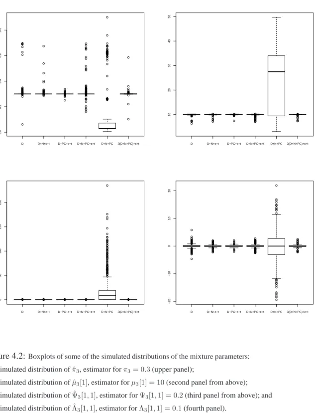
The distributions of the estimators for the model parameters can be represented through
some box plots, and some of them are shown in Figure 4.2, namely with reference toπˆ3 (upper
Table 4.4: Case with trimming and constraints.
Bias as the sum of absolute deviations, followed by MSE (in parentheses) of the parameter estimators
ˆ
πi,µˆi,Ψˆi,Λˆi, for i = 1,2,3 when dealing with different datasets. The column labels refer to the different scenarios, namely D stays for data, D+N stays for data and added noise, D+PC stays for data and pointwise
contamination, D+N+PC stays for data with added noise and pointwise contamination.
D D+N D+PC D+N+PC 3*(D+N+PC)
ˆ
τ1 0.0151 0.0002 0.0011 0 0.0006
(0.0002) (0) (0) (0) (0)
ˆ
τ2 0.0195 0.0014 0.0011 0.0034 0.0006
(0.0004) (0) (0) (0) (0)
ˆ
τ3 0.0044 0.0012 0.0001 0.0034 0.0001
(0) (0) (0) (0) (0)
ˆ
µ1 0.006 0.010 0.017 0.006 0.001
(0.117) (0.159) (0.215) (0.226) (0.038)
ˆ
µ2 0.006 0.004 0.002 0.007 0.009
(0.190) (0.219) (0.165) (0.703) (0.158)
ˆ
µ3 0.008 0.020 0.004 0.062 0.018
(0.177) (0.302) (0.154) (0.787) (0.231)
ˆ
Ψ1 0.013 0.029 0.026 0.032 0.022
(0.010) (0.025) (0.024) (0.035) (0.009)
ˆ
Ψ2 0.066 0.044 0.045 0.046 0.042
(0.089) (0.082) (0.081) (0.102) (0.058)
ˆ
Ψ3 0.066 0.072 0.075 0.076 0.075
(0.108) (0.158) (0.154) (0.178) (0.158)
ˆ
Λ1 0.516 0.512 0.516 0.546 0.524
(13.168) (14.828) (12.992) (14.711) (13.674)
ˆ
Λ2 0.568 0.569 0.569 0.586 0.578
(11.049) (12.311) (12.036) (13.875) (12.832)
ˆ
Λ3 0.330 0.353 0.354 0.341 0.342
(9.377) (11.164) (12.259) (13.069) (13.064)
in a direct comparison, that the estimation algorithm with adequate trimming and constraints
is able to resist all type of outlying data. In each panel, the first boxplot on the left provides
the benchmark of the following five ones, as it shows the distribution of the estimator when the
data has been drawn from the mixture. The second boxplot (from left to right) in each panel
shows the distribution of the estimator when we employ constraints and trimming along the
estimation on data and added uniform noise. The third boxplot refers to the case in which we
deal with data and pointwise contamination, and the good results are obtained because we are
employing constraints and trimming. The fourth box plot has been obtained when considering
effects of noise and pointwise contamination when the estimation procedure does not employ
constraints and trimming. Finally the sixth box plot in all panels reports the case of robust
estimation performed on a triple sample size, still with noise and pointwise contamination.
4.2
Real data: the AIS data set
As an illustration, we apply the proposed technique to the Australian Institute of Sports (AIS)
data, which is a famous benchmark dataset in the multivariate literature, originally reported
by Cook and Weisberg (1994) and subsequently analyzed by Azzalini and Dalla Valle (1996),
among many other authors. The dataset consists ofp= 11physical and hematological
measure-ments on 202 athletes (100 females and 102 males) in different sports, and is available within
the R package sn (Azzalini, 2011). The observed variables are: red cell count (RCC), white cell
count (WCC), Hematocrit (Hc), Hemoglobin (Hg), plasma ferritin concentration (Fe), body
mass index, weight/height2 (BMI), sum of skin folds (SSF), body fat percentage (Bfat), lean
body mass (LBM), height, cm (Ht), weight, kg (Wt), a part from Sex and kind of Sport. A
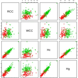
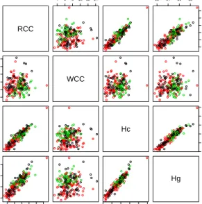
partial scatterplot of the AIS dataset is given in Figure 4.3, and Table 4.5 provides summary
information.
Table 4.5: Summary information for the AIS dataset
female athletes male athletes
min Q1 Me Q3 max mean min Q1 Me Q3 max mean
RCC 3.8 4.2 4.4 4.5 5.3 4.4 4.1 4.9 5.0 5.2 6.7 5.0
W CC 3.3 5.8 6.7 8.0 13.3 7.0 3.9 6.0 7.1 8.4 14.3 7.2
Hc 35.9 38.3 40.6 42.3 47.1 40.5 40.3 44.2 45.5 46.8 59.7 45.6
Hg 11.6 12.7 13.5 14.3 15.9 13.6 13.5 14.9 15.5 15.9 19.2 15.6
F e 12.0 36.0 50.0 71.5 182.0 57.0 8.0 55.0 89.5 123.5 234.0 96.4
BM I 16.8 20.3 21.8 23.4 31.9 22.0 19.6 22.3 23.6 25.2 34.4 23.9
SSF 33.8 59.3 81.8 107.4 200.8 87.0 28.0 37.5 47.7 58.1 113.5 51.4
Bf at 8.1 13.2 17.9 21.4 35.5 17.8 5.6 7.0 8.6 10.0 19.9 9.3
LBM 34.4 51.9 54.9 59.4 73.0 54.9 48.0 68.0 74.5 80.8 106.0 74.7
Ht 148.9 171.0 175.0 179.7 195.9 174.6 165.3 179.7 185.6 191.0 209.4 185.5
W t 37.8 60.1 68.1 74.4 96.3 67.3 53.8 73.9 83.0 90.3 123.2 82.5
Our purpose is to provide a model for the entire dataset, and classify athletes by Sex. Let
D D+N+c+t D+PC+c+t D+N+PC+c+t D+N+PC 3(D+N+PC)+c+t
0.0
0.2
0.4
0.6
0.8
D D+N+c+t D+PC+c+t D+N+PC+c+t D+N+PC 3(D+N+PC)+c+t
10
20
30
40
50
D D+N+c+t D+PC+c+t D+N+PC+c+t D+N+PC 3(D+N+PC)+c+t
0
50
100
150
200
D D+N+c+t D+PC+c+t D+N+PC+c+t D+N+PC 3(D+N+PC)+c+t
−20
−10
0
10
20
Figure 4.2:Boxplots of some of the simulated distributions of the mixture parameters:
the simulated distribution ofπˆ3, estimator forπ3= 0.3(upper panel);
the simulated distribution ofµˆ3[1], estimator forµ3[1] = 10(second panel from above); the simulated distribution ofΨˆ3[1,1], estimator forΨ3[1,1] = 0.2(third panel from above); and the simulated distribution ofΛˆ3[1,1], estimator forΛ3[1,1] = 0.1(fourth panel).
The labels on the horizontal axis refers to the six settings, namely “D” stays for data, “D+N” stays for data and
added noise, “D+N+PC” stays for data with added noise and pointwise contamination, while “c + t” has been
RCC
4 6 8 1012 14 12 14 16 18
4.0
5.0
6.0
4
6
8
10
12
14
WCC
Hc
35
40
45
50
55
60
4.0 5.0 6.0
12
14
16
18
35 40 45 50 55 60
Hg
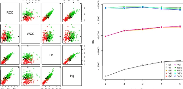
Figure 4.3:Scatterplot of some pairs of the AIS variables (female data in red, male in blue)
package in R. The routine mclustBIC fits a set of normal mixture models, on the base of the
parameters you set in its call. We considered from 1 to 9 components in the mixture and different
patterns for the covariance matrices, from the more constrained homoscedastic model, to the
more general heteroscedastic one. After the estimation, mclustBIC provides a model selection
procedure based on the BIC, a well-known penalized likelihood criterium. In Figure 4.4 the
BIC values for each kind of model are shown, and for each choice of the number of mixture
components. The three letters in the acronym of the models stand respectively for the volume,
the shape and orientation of the ellipsoids of equal probability of the components, which could
be Equal (hence E) or Variable (V) across the components. Notice that the shape may also
be Isotropic (hence the letter I denotes spherical ellipsoids), in this case also the orientation is
the same. Hence, we see that Mclust suggests an EEV model (ellipsoidal, equal volume and
shape, different orientation of the component scatters) withG = 2components, providing the
highest BIC value, i.e. BIC = −10251.6. Now, if we employ the model suggested by Mclust
to classify AIS data, we obtain 18 misclassified units, i.e., a misclassification error equal to
18/202 = 9.4%. In Figure 4.4 we can see the classification results. Surely this is not an easy
dataset for classification, due to the apparent class overlapping we saw in the first scatterplot in
Figure 4.3.
ex-RCC
4 6 8 10 12 14 12 14 16 18
4.0
5.0
6.0
4
6
8
10
12
14
WCC
Hc
35
40
45
50
55
60
4.0 5.0 6.0
12
14
16
18
35 40 45 50 55 60
Hg
1 2 3 4 5
−18000
−16000
−14000
−12000
−10000
Number of components
BIC
EII VII EEI VEI EVI
VVI EEE EEV VEV VVV
Figure 4.4:The classification of AIS data obtained through the best model from Mclust (left panel, with female
data in red, male in blue, misclassified units as black circlecrosses), and the graphical tool for model selection
(right panel)
ists among the hematological and physical measurement. Therefore we fit mixtures of factor
analyzers, assuming the existence of some underlying unknown factors (like nutritional status,
hematological composition, overweight status indices, and so on) which jointly explains the
observed measurements. Through the underlying factors, we aim at finding a perspective on
data which disentangle the overlapping components. To avoid variables having a greater impact
in the model (which is not affine equivariant) due to different scales, before performing the
es-timation, the variables have been standardized to have zero mean and unit standard deviation.
We begin by adopting the pGmm package from R, that fits mixtures of factors analyzers with
patterned covariances. Parsimonious Gaussian mixtures are obtained by constraining the
load-ingΛj and the errors Ψj to be equal or not among the components. We employed the routine
pGmmEM, considering from 1 to 9 components, and number of underlying factors dranging
from 1 to 6, with 30 different random initialization, to provide the best iteration (in terms of
BIC) for each case. The best model is a CUU mixture model with d = 4 factors and G = 3
components, withBIC =−3127.424. CUU means Constrained loading matricesΛj = Λand
Unconstrained error matricesΨg =ωg∆g, where ∆g are normalized diagonal matrices andωg
is a real value varying across components. Using this model to classify athletes, we got 109
RCC
4 6 8 101214 12 14 16 18
4.0
5.0
6.0
4
6
8
10
12
14
WCC
Hc
35
40
45
50
55
60
4.0 5.0 6.0
12
14
16
18
35 40 45 50 55 60
Hg
Figure 4.5: The classification of AIS data obtained through the best UUU model from pGmm withG= 2and
d= 4(female data in red, male in green, misclassified units in black)
As a second attempt using pGmm, we estimated a UUU model by setting G = 2
com-ponents, and d = 6. The acronym UUU means that we leave the estimation of loadings Λj
and errors Ψj unconstrained. Based on 30 random starts, the best UUU model had BIC =
−3330.306, and the consequent classification of the AIS dataset produces 72 misclassifies units
(misclassification error=35.6%), that are visualized in Figure 4.5.
Finally, we want to show the performances of our trimmed and constrained estimation for
MFA on the AIS data. All the results are generated by the procedure described in Section 3.2,
are based on 30 random initializations and returning the best obtained solution of the
parame-ters, in terms of highest value of the final likelihood.
Table 4.6: Trimmed and constrained MFA estimation on the AIS data set (best results over 30 random
initializations). Misclassification errorη(in percentage) under different settings
cnoise 1010 45 1010 45 1010 45 1010 45
cload 1010 1010 10 10 1010 1010 10 10
α 0 0 0 0 0.05 0.05 0.05 0.05
η 0.0891 0.1881 0.4554 0.0842 0.1039 0.1782 0.4505 0.0149
We see that the best solution, with only 3 misclassified points, has been obtained by
F F F F F F F F F F X F F F F F F F F F F F F F F F F F F F F F F F F F F F F F F F F F F F F F F F F F F F F X F F F F F F F F F F F F F O F F O F X F F F F F F F F F F F
F FF
F F F X F F FF F X F M M M M M M M M M M M M M M M M M M M M O M M M M M M M M M M M X M M M M M M M M MM M M M M M M MM MM M
M M M M M X M M X M M X M M M M M M M M M M M X M M M M M M M M M M M M M M M M M M M M M M M M
−2 −1 0 1 2 3 4
−1 0 1 2 3 4 BMI SSF F F F F F F F F F F F F F F F F F F F F F F F F F F F F F F F F F F F F F F F F F F F F F F F F F F F F F F F F F F F F F F F F F F F F F F F F F F F F F F F F F F F F F F
F FF
F F F F F F FF F F F M M M M M M M M M O M M M M O M M M M M O M M M M M M M M M M M O M M M M M M M M MM M O O M M M MM MM M
M M M M M O M O O M M M M M M M M M M M M M M O O M M O M O O M M M M O M O M M M O M O M M M M
−2 −1 0 1 2 3 4
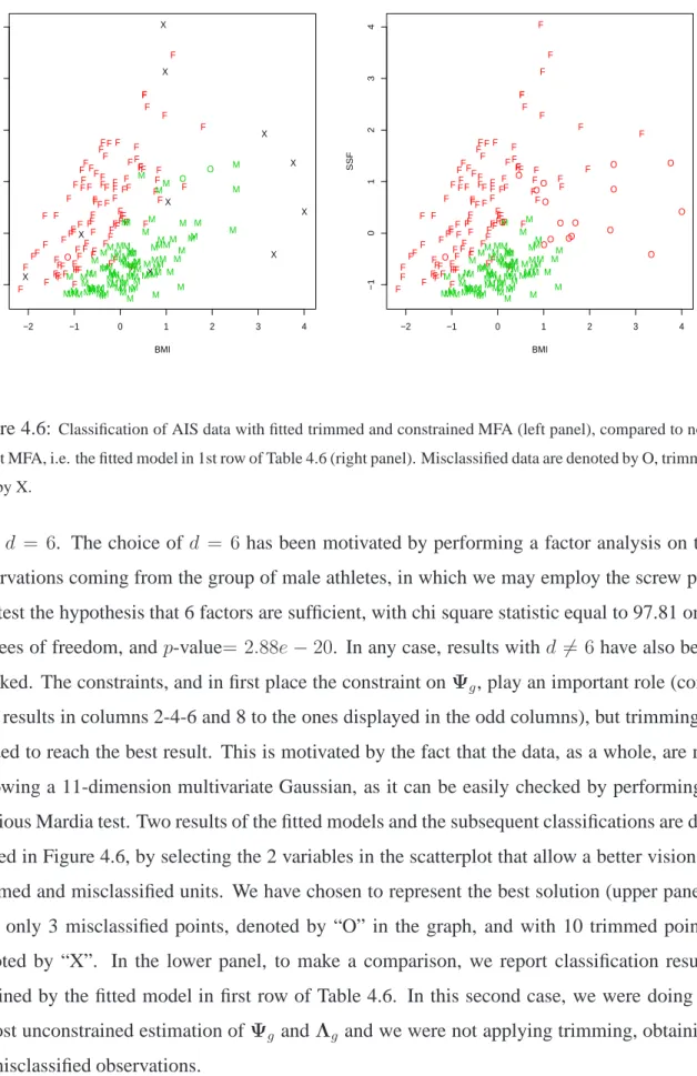
−1 0 1 2 3 4 BMI SSF
Figure 4.6: Classification of AIS data with fitted trimmed and constrained MFA (left panel), compared to
non-robust MFA, i.e. the fitted model in 1st row of Table 4.6 (right panel). Misclassified data are denoted by O, trimmed
data by X.
with d = 6. The choice of d = 6has been motivated by performing a factor analysis on the
observations coming from the group of male athletes, in which we may employ the screw plot
and test the hypothesis that 6 factors are sufficient, with chi square statistic equal to 97.81 on 4
degrees of freedom, andp-value= 2.88e−20. In any case, results withd 6= 6have also been
checked. The constraints, and in first place the constraint onΨg, play an important role
(com-pare results in columns 2-4-6 and 8 to the ones displayed in the odd columns), but trimming is
needed to reach the best result. This is motivated by the fact that the data, as a whole, are not
following a 11-dimension multivariate Gaussian, as it can be easily checked by performing a
previous Mardia test. Two results of the fitted models and the subsequent classifications are
dis-played in Figure 4.6, by selecting the 2 variables in the scatterplot that allow a better vision of
trimmed and misclassified units. We have chosen to represent the best solution (upper panel),
with only 3 misclassified points, denoted by “O” in the graph, and with 10 trimmed points,
denoted by “X”. In the lower panel, to make a comparison, we report classification results
obtained by the fitted model in first row of Table 4.6. In this second case, we were doing an
almost unconstrained estimation ofΨg andΛg and we were not applying trimming, obtaining
18 misclassified observations.
misclas-sified units are among female athletes, one is among male athletes. The density of the mixture
components for the observation in position 73 are close (0.000021 and 0.00034), while for the
other two observations they are neatly different.
Finally, we recall that trimmed observations were discarded to provide robustness to the
parameter estimation. After estimating the model, hence, it makes sense to classify also these
observations. The trimmed observations are in rows 11, 56, 75, 93, 99, 133, 160, 163, 166,
178, and if we assign them by the Bayes rule to the component g having greater value of
Dg(x;θ) =φp x;µg,ΛgΛ′g +Ψg
πg, we classify the first five in the female group of athletes,
and the second group of five in the male group. This means that all the trimmed observations
have been assigned to their true group. Table 4.7 shows the details of the classification, and
Figure 4.7 plots the final result of the robust model fitting.
Table 4.7: Trimmed units in the AIS data set and their final classification
unit D1(x;θ) =φp x;µ1,Λ1Λ′1+Ψ1
π1 D2(x;θ) =φp x;µ2,Λ2Λ′2+Ψ2
π2 Sex
11 1.4 e-15 9.2 e-20 F
56 7.2 e-08 4.5 e-25 F
75 5.2 e-09 1.2 e-11 F
93 1.7 e-07 1.0 e-10 F
99 1.2 e-09 6.4 e-70 F
133 9.8 e-85 3.2 e-12 M
160 9.9 e-74 1.5 e-08 M
163 9.9 e-87 2.0 e-08 M
166 2.2 e-16 1.4 e-13 M
178 3.1 e-23 3.8 e-13 M
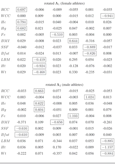
As a last analysis on AIS dataset, we are interested in factor interpretation.
The rotated factor loading matrices have been obtained by employing a Gradient
Projec-tion algorithm, available through the R package GPArotaProjec-tion (Bernaards and Jennrich, 2005;
Browne, 2001). We opted for an oblimin transformation, which yielded results shown in Table
4.8. We observe that the two groups highlight the same factors, while in a slightly different
order of importance. The first factor for the group of observations for female athletes, may be
labelled as a hematological factor, with a very high loading onHc, followed byRCC andHg.
The second factor, loading heavily onHt, and in a lesser extent onW tandLBM, may be
F F F F F F F F F F F F F F F F F F F F F F F F F F F F F F F F F F F F F F F F F F F F F F F F F F F F F F F F F F F F F F F F F F F F F O F F O F F F F F F F F F F F F F
F FF
F F F F F F FF F F F M M M M M M M M M M M M M M M M M M M M O M M M M M M M M M M M M M M M M M M M M MM M M M M M M MM MM M
M M M M M M M M M M M M M M M M M M M M M M M M M M M M M M M M M M M M M M M M M M M M M M M M
−2 −1 0 1 2 3 4
−1 0 1 2 3 4 BMI SSF
Figure 4.7: Classification of AIS data after classifying also trimmed observations. The three misclassified points
are denoted by O, and they represent only1.5%of the data.
BMI, respectively. The fifth factor can be viewed as a overweight assessment index sinceSSF
andBf at load highly on it. The sixth factor is related only toW CC. Noticing thatW CC is
not joined into the hematological factor, we observe that the specific role of lymphocytes, cells
of the immune system that are involved in defending the body against both infectious disease
and foreign invaders, seems to be pointed out. Analogous comments may be done on the factor
loadings for the group of male athletes.
5
Concluding remarks
In this paper we propose a robust estimation for the mixture of Gaussian factors model. To
resist pointwise contamination and sparse outliers that could arise in data collection, we adopt
and incorporate a trimming procedure along the iterations of the EM algorithm. The key idea is
that a small portion of observations which are highly unlikely to occur, under the current fitted
model assumption, are discarded from contributing to the parameter estimates. Furthermore, to
reduce spurious solutions and avoid singularities of the likelihood, we implement a constrained
ML estimation for the component covariances. Results from Monte Carlo experiments show
that bias and MSE of the estimators in several cases of contaminated data are comparable to
Table 4.8:Factor loadings in the AIS data set
rotatedΛ1(female athletes)
RCC 0.697 -0.006 -0.009 -0.055 0.001 -0.035
W CC 0.000 0.009 0.000 -0.015 0.012 −0.941
Hc 0.794 -0.015 0.040 -0.004 0.010 0.026
Hg 0.682 0.021 -0.025 0.047 -0.002 0.007
F e 0.002 -0.005 −0.510 0.003 -0.004 0.000
BM I 0.029 -0.008 0.023 0.644 -0.316 -0.057
SSF -0.040 -0.012 -0.037 0.033 −0.889 -0.017
Bf at 0.014 -0.024 0.013 -0.007 −0.826 0.008
LBM 0.022 −0.419 0.020 0.295 0.054 -0.025
Ht 0.020 −0.924 0.023 -0.128 -0.076 -0.002
W t 0.029 −0.468 0.023 0.330 -0.235 -0.031
rotatedΛ2(male athletes)
RCC -0.033 0.663 0.077 -0.015 -0.025 -0.053
W CC 0.003 -0.004 0.024 -0.003 1.024 0.013
Hc 0.048 0.622 -0.008 0.005 0.036 -0.048
Hg -0.002 0.604 -0.051 0.009 0.001 0.079
F e 0.010 -0.006 0.027 1.103 -0.004 0.008
BM I -0.371 0.109 −0.656 0.074 0.070 -0.261
SSF −0.616 0.002 0.009 -0.001 0.015 -0.026
Bf at −0.610 -0.009 0.003 0.007 -0.000 0.040
LBM 0.036 0.071 -0.344 0.037 0.053 −0.885
Ht 0.036 0.005 0.170 -0.022 0.009 −1.157
W t -0.222 0.071 -0.357 0.042 0.056 −0.884
robust estimation leads to better classification and provides direct interpretation of the factor
loadings.
Further investigations are needed to tune the choice of the parameters, such as the
por-tion of trimming data and the values of the constraints.Though interesting, this issue is beyond
the scope of the present paper. Surely, the researcher may specify the partial information he
may have about the shape of the expected clusters from the data at hand, hence providing
a part of these parameters. Then, data-dependent diagnostic based on trimmed BIC notions
conveniently adapted to the specific case, could assist in taking appropriate choices for the rest
of the parameters. The encouraging results here obtained suggest a deeper discussion of these
implementation details in a future work.
Acknowledgements
This research is partially supported by the Spanish Ministerio de Ciencia e Innovaci´on, grant
MTM2011-28657-C02-01, by Consejer´ıa de Educaci´on de la Junta de Castilla y Le´on, grant VA212U13, and by grant FAR 2013
from the University of Milano-Bicocca.
References
Azzalini A., Dalla Valle A., The multivariate skew-normal distribution, Biometrika, 83 (4), 715–726, (1996).
Baek J., McLachlan G., Flack L., Mixtures of Factor Analyzers with Common Factor Loadings: Applications to the
Clustering and Visualization of High-Dimensional Data, IEEE Transactions on Pattern Analysis and Machine
Intelligence, 32 (7), 1298 –1309, (2010).
Baek J., McLachlan G., Mixtures of common t-factor analyzers for clustering high-dimensional microarray data,
Bioinformatics, 27 (9), 1269–1276, (2011).
Bernaards C. A., Jennrich R. I. , Gradient projection algorithms and software for arbitrary rotation criteria in factor
analysis, Educational and Psychological Measurement, 65 (5), 676–696, (2005).
Bickel D.R., Robust cluster analysis of microarray gene expression data with the number of clusters determined
biologically, Bioinformatics, 19 (7), 818–824, (2003).
Bishop C. M., Tipping M. E., A Hierarchical Latent Variable Model for Data Visualization, IEEE Transactions on
Pattern analysis and Machine Intelligence , 20, 281–293, (1998).
Browne M. W., An overview of analytic rotation in exploratory factor analysis, Multivariate Behavioral Research,
36 (1), 111–150, (2001).
Campbell J., Fraley C., Murtagh F., Raftery A., Linear flaw detection in woven textiles using model-based
cluster-ing, Pattern Recognition Letters, 18 (14), 1539 – 1548, (1997).
Cook R. D., Weisberg S., An introduction to regression graphics, vol. 405, John Wiley & Sons, 1994.
Coretto P., Hennig C., Maximum likelihood estimation of heterogeneous mixtures of Gaussian and uniform
distri-butions, Journal of Statistical Planning and Inference, 141 (1) 462–473, (2011) .
Fokou´e E., Titterington D., Mixtures of factor analysers. Bayesian estimation and inference by stochastic
Fraley C., Raftery A. E., How Many Clusters? Which Clustering Method? Answers Via Model-Based Cluster
Analysis, Computer Journal, 41 (8), 578–588, (1998).
Fritz H., Garc´ıa-Escudero L., Mayo-Iscar A., A fast algorithm for robust constrained clustering, Computational
Statistics & Data Analysis, (61), 124–136, (2013).
Gallegos M., Ritter G., Trimmed ML estimation of contaminated mixtures, Sankhya (Ser. A), (71), 164–220,
(2009).
Garc´ıa-Escudero L. A., Gordaliza A., Matr´an C., Mayo-Iscar A., A General Trimming Approach to Robust Cluster
Analysis, The Annals of Statistics, 36 (3) 1324–1345 (2008).
Garc´ıa-Escudero L. A., Gordaliza A., Matr´an C., Mayo-Iscar A., Exploring the Number of Groups in Robust
Model-Based Clustering, Statistics and Computing, 21 (4), 585–599, (2011).
Garc´ıa-Escudero L., Gordaliza A., Mayo-Iscar A., A constrained robust proposal for mixture modeling avoiding
spurious solutions, Advances in Data Analysis and Classification, 8 (1), 27–43, (2014).
Ghahramani Z., Hilton G., The EM algorithm for mixture of factor analyzers, Techical Report CRG-TR-96-1,
(1997).
Greselin F., Ingrassia S., Maximum likelihood estimation in constrained parameter spaces for mixtures of factor
analyzers, Statistics and Computing, 25, 215–226, (2015).
Hathaway R., A constrained formulation of maximum-likelihood estimation for normal mixture distributions, The
Annals of Statistics, 13 (2), 795–800, (1985).
Hennig C., Breakdown points for maximum likelihood-estimators of location-scale mixtures, Annals of Statistics,
32, 1313–1340, (2004).
Ingrassia S., A likelihood-based constrained algorithm for multivariate normal mixture models, Statistical Methods
& Applications, 13, 151–166, (2004).
Ingrassia S., Rocci R., Constrained monotone EM algorithms for finite mixture of multivariate Gaussians,
Compu-tational Statistics & Data Analysis, 51, 5339–5351, (2007).
Lin T.-I., McNicholas P. D., Ho H. J., Capturing patterns via parsimonious t mixture models, Statistics &
Proba-bility Letters, 88, 80–87, (2014).
Maitra R., Clustering Massive Datasets With Application in Software Metrics and Tomography, Technometrics,
43 (3), 336–346, (2001).
Maitra R., Initializing partition-optimization algorithms, IEEE/ACM Transactions on Computational Biology and
Bioinformatics 6 (1) 144–157, (2009).
McLachlan G., Peel D., Robust cluster analysis via mixtures of multivariatet-distributions, in: A. Amin, D. Dori, P. Pudil, H. Freeman (Eds.), Advances in Pattern Recognition, vol. 1451 of Lecture Notes in Computer Science,
Springer Berlin - Heidelberg, 658–666, (1998).
McLachlan G., Peel D., Mixtures of factor analyzers, in: Proceedings of the Seventeenth International Conference
on Machine Learning, P. Langley (Ed.)., San Francisco: Morgan Kaufmann, 599–606, (2000a).
McLachlan G. J., Peel D., Finite Mixture Models, John Wiley & Sons, New York, (2000b).
McNicholas P., Murphy T., Parsimonious Gaussian mixture models, Statistics and Computing, 18 (3), 285–296,
(2008).
Neykov N., Filzmoser P., Dimova R., Neytchev P., Robust Fitting of Mixtures Using the Trimmed Likelihood
Estimator, Computational Statistics & Data Analysis, 52 (1), 299–308, (2007).
R. D. C. Team, R: A Language and Environment for Statistical Computing, R Foundation for Statistical Computing,
Vienna, Austria, URLhttp://www.R-project.org, (2013).
Rousseeuw P. J., Van Driessen K., A Fast Algorithm for the Minimum Covariance Determinant Estimator,
Tech-nometrics, 41, 212–223, (1999).
Steane M. A., McNicholas P. D., R. Y. Yada, Model-based classification via mixtures of multivariate t-factor
analyzers, Communications in Statistics-Simulation and Computation, 41 (4), 510–523, (2012).
Stewart C. V., Robust parameter estimation in computer vision, SIAM review, 41 (3), 513–537, (1999).
Tipping M. E., Bishop C. M., Mixtures of probabilistic principal component analyzers, Neural computation, 11 (2),