Why Do Computer Methods For Grounding
Analysis Produce Anomalous Results?
Ferm´ın Navarrina, Ignasi Colominas, Member, IEEE, and Manuel Casteleiro
Abstract— Grounding systems are designed to guarantee
per-sonal security, protection of equipments and continuity of power supply. Hence, engineers must compute the equivalent resistance of the system and the potential distribution on the earth surface when a fault condition occurs [1], [2], [3]. While very crude approximations were available until the 70’s, several computer methods have been more recently proposed on the basis of practice, semi-empirical works and intuitive ideas such as super-position of punctual current sources and error averaging [1], [3], [4], [5], [6]. Although these techniques are widely used, several problems have been reported. Namely: large computational re-quirements, unrealistic results when segmentation of conductors is increased, and uncertainty in the margin of error [2], [5].
A Boundary Element formulation for grounding analysis is presented in this paper. Existing computer methods such as APM are identified as particular cases within this theoretical framework. While linear and quadratic leakage current elements allow to increase accuracy, computing time is reduced by means of new analytical integration techniques. Former intuitive ideas can now be explained as suitable assumptions introduced in the BEM formulation to reduce computational cost. Thus, the anomalous asymptotic behaviour of this kind of methods is mathematically explained, and sources of error are rigorously identified.
Index Terms— Anomalous results, average potential method,
boundary element methods, boundary integral equations, com-puter methods for grounding analysis, convergence of numerical methods, fault currents, grounding, power system protection.
I. INTRODUCTION
F
AULT currents dissipation into the earth can be modelled by means of Maxwell’s Electromagnetic Theory [7], [8], [9]. Constraining the analysis to the electrokinetic steady-state response, and neglecting the resistivity of the earthing electrode, the 3D problem associated to an electrical current derivation to earth can be written asdiv(σσσσσ) = 0σσσσσσσσσ in E, being σσσσσσσσσσσσσσ=−γγγγγγγγγγγγγγ grad(V) σ
σ σ σσσσ σ σ σσσ σ
σtnnnnnnnnnnnnnnE= 0 in Γ
E, V =VΓ in Γ,
V →0 if |xxxxxxxxxxxxxx| → ∞, (1)
where E is the earth andγγγγγγγγγγγγγγ its conductivity tensor,ΓE is the earth surface and nnEnnnnnnnnnnnn its normal exterior unit field, and Γ is the earthing electrode surface [10], [11], [12]. The solution to this problem gives the potential V(xxx)xxxxxxxxxxx and the current density σσσ(xσσσσσσσσσσσxxx)xxxxxxxxxx at an arbitrary pointxxxxxxxxxxxxxxinE when the earthing electrode is energized to the so-called Ground Potential RiseVΓ relative
to remote earth.
Manuscript received November 13, 2000.
F. Navarrina, I. Colominas and M. Casteleiro are with the Department of Applied Mathematics, Civil Engineering School, University of A Coru˜na, Campus de Elvi˜na 15071 A Coru˜na, SPAIN (e-mail: [email protected], web page:<http://caminos.udc.es/gmni>).
Publisher Item Identifier S 0000–0000(00)00000–0.
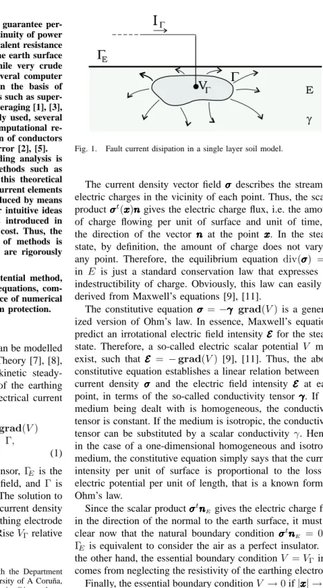
Fig. 1. Fault current disipation in a single layer soil model.
The current density vector field σσσσσσσσσσσσσσdescribes the stream of electric charges in the vicinity of each point. Thus, the scalar productσσσσσσσσσσσσσσt(xxx)nxxxxxxxxxxxnnnnnnnnnnnnngives the electric charge flux, i.e. the amount of charge flowing per unit of surface and unit of time, in the direction of the vector nnnnnnnnnnnnnn at the point xxxxxxxxxxxxxx. In the steady state, by definition, the amount of charge does not vary at any point. Therefore, the equilibrium equation div(σσσσσσσσσσσσσ) = 0σ in E is just a standard conservation law that expresses the indestructibility of charge. Obviously, this law can easily be derived from Maxwell’s equations [9], [11].
The constitutive equationσσσσσσσσσσσσσσ=−γγγγγγγγγγγγγγ grad(V) is a general-ized version of Ohm’s law. In essence, Maxwell’s equations predict an irrotational electric field intensityEEEEEEEEEEEEEE for the steady state. Therefore, a so-called electric scalar potential V must exist, such that EEEEEEEEEEEEEE = −grad(V) [9], [11]. Thus, the above constitutive equation establishes a linear relation between the current density σσσσσσσσσσσσσσ and the electric field intensity EEEEEEEEEEEEEE at each point, in terms of the so-called conductivity tensorγγγγγγγγγγγγγγ. If the medium being dealt with is homogeneous, the conductivity tensor is constant. If the medium is isotropic, the conductivity tensor can be substituted by a scalar conductivity γ. Hence, in the case of a one-dimensional homogeneous and isotropic medium, the constitutive equation simply says that the current intensity per unit of surface is proportional to the loss of electric potential per unit of length, that is a known form of Ohm’s law.
Since the scalar productσσσσσσσσσσσσσσtnnnnnnnnnnnnnnEgives the electric charge flux in the direction of the normal to the earth surface, it must be clear now that the natural boundary condition σσσσσσσσσσσσσσtnnEnnnnnnnnnnnn = 0 in ΓE is equivalent to consider the air as a perfect insulator. On the other hand, the essential boundary conditionV =VΓ inΓ
V must satisfy some theoretical regularity requirements at infinity. These so-called “normal conditions” are made explicit in Appendix I [7], [8].
In these terms, the leakage current density σ(ξξξξξξξξξξξξξξ) at an arbitrary pointξξξξξξξξξξξξξξon the earthing electrode surface, the ground currentIΓ(total surge current being leaked into the earth) and
the equivalent resistance of the earthing system Req, can be written as are proportional to the GPR, the assumption VΓ = 1 is not
restrictive at all and it will be used from now on.
For most practical purposes, the assumption of homoge-neous and isotropic soil can be considered acceptable [1], and the tensorγγγγγγγγγγγγγγ can be substituted by a meassured apparent scalar conductivity γ (see figure 1). Otherwise, a multi-layer model can be accepted without risking a serious calculation error [13], [14]. Since the kind of techniques described in this paper can be extended to multi-layer soil models [15], further discussion is restricted to uniform soils. Hence, problem (1) reduces to the Laplace equation with mixed boundary conditions [7], [8]. If one further assumes that the earth surface is horizontal (see Appendix I), symmetry allows to rewrite (1) in terms of a Dirichlet Exterior Problem [16].
This kind of problems has been rigorously studied [17], and its solution can be obtained in many technical applications by means of the Finite Diference or the Finite Element methods. But that is not our case. In most substation grounding systems, the buried earthing electrode (grounding grid) consists of a number of interconnected bare cylindrical conductors, which ratio diameter/lenght is relatively small (≈ 10−3). Since domainE is half-infinite and the electrode must be excluded, the adequate discretization of E requires an extremely large number of degrees of freedom. Thus, the prohibitive comput-ing requirements preclude the use of FD or FE methods in practice [18].
On the other hand, two basic goals must be achieved in a grounding system design: human safety must be preserved (by limiting step and touch voltages), and integrity of equipment and continuity of service must be guaranteed (by ensuring fault currents dissipation into the earth) when a fault condition occurs [1], [2], [11]. Since computation of potential is only required on the earth surfaceΓE, and the equivalent resistance can be easily obtained in terms of the leakage current (2), a Boundary Element approach [19] seems to be the right choice [10], [11], [12].
II. VARIATIONALSTATEMENT OF THEPROBLEM
Applying Green’s Identity [17] to (1), one gets the following expression (see Appendix I) for the potentialV inE, in terms of the unknown leakage current σ[10], [11], [12]
V(xxxxxxxxxxxxx) =x 1 4πγ
Z Z
ξξξξξξξξξξξξξξ∈Γ
k(xxx, ξξξξξξξξξξξξξξ)xxxxxxxxxxx σ(ξξξξξξξξξξξξξξ)dΓ, (3)
with the weakly singular kernel
k(xxxxxxxxxxxxxx, ξξξξξξξξξξξξξξ) =
whereξξξξξξξξξξξξξξ0is the symmetric ofξξξξξξξξξξξξξξwith respect to the earth surface. Since (3) holds on the earthing electrode surface [11], the boundary condition VΓ = 1 leads to the Fredholm integral
equation of the first kind onΓ
1− 1
4πγ
Z Z
ξξξξξξξξξξξξξξ∈Γ
k(χχχχ, ξξξξξξξξξξξξξξ)χχχχχχχχχχ σ(ξξξξξξξξξξξξξξ)dΓ = 0 ∀χχχχχχχχχχχχχχ∈Γ, (5)
which solution is the unknown leakage current density σ. Equation (5) can be written in the weaker variational (or weighted residuals) form [19], [20]
Z Z so-called test (or weighting) functions onΓ[10], [11], [12].
It seems quite clear that the weak form (6) is a consequence of the original (or strong) form (5) of the problem. The reverse is not obvious, but it can be proved. The basic idea is quite simple: roughly speaking, weak form (6) must be satisfied for any selected test functionw(χχχχχχχχχχχχχχ), and this will not be possible unless strong form (5) is fulfilled. In fact, both forms of the problem can be proved to be equivalent [19], [20] as a general rule.
Weak form (6) will be our starting point to obtain an approximate solution to the original problem (1) by means of the Boundary Element Method. Following the subsequent developments will be fairly straightforward for those readers who are familiar with the Finite Element basic technology [20], [19], [9]. The essential idea is to approximate variational statement (6) in a finite-dimensional context. First, we shall substitute the exact solutionσ(ξξξξξξξξξξξξξξ)by a discretized approxima-tionσh(ξξξξξξξξξξξξξξ)in terms of a set of unknown parameters. And, sec-ond, we shall discretize the space of test functions in a similar way. Our purpose is to reduce the approximated problem to a well posed linear system, with the same number of degrees of freedom (unknown parameters) as discretized equations. We shall also discretize the geometry of the boundary, which is usual in this kind of methods, with the aim of simplifying and systematizing the integration tasks.
2D Boundary Element General Formulation
For a given set {Ni(ξξξξξξξξξξξξξξ)} of N so-called trial (or interpo-lating) functions [19], [20] defined on Γ, and for a given set
{Γα} ofM 2D boundary elements (portions of the electrode surface), the unknown leakage current density σ and the electrode surfaceΓ can be discretized in the form
σ(ξξξξξξξξξξξξξξ)≈σh(ξξξξξξξξξξξξξξ) =
Then, a discretized form of (3) can be written as
x
^ x
s( )^x
C( )^x
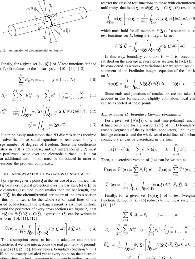
Fig. 2. Assumption of circumferential uniformity.
Finally, for a given set{wj(ξξξξξξξξξξξξξξ)}ofN test functions defined on Γ, (6) reduces to the linear system [10], [11], [12]
N
It can be easily understood that 2D discretizations required to solve the above stated equations in real cases imply a large number of degrees of freedom. Since the coefficients matrix in (10) is not sparse, and 2D integration in (12) must be performed twice over the electrode surface, it is clear that additional assumptions must be introduced in order to overcome the problem complexity.
III. APPROXIMATED1D VARIATIONALSTATEMENT
For a given generic pointξξξξξξξξξξξξξξat the surface of a cylindrical bar, letbξξξξξξξξξξξξξξbe its orthogonal projection over the bar axis, letφ(bξξξξξξξξξξξξξξ)be the diameter (assumed much smaller than the bar length) and let C(bξξξξξξξξξξξξξξ)be the circumferential perimeter of the cross section at this point. Let L be the whole set of axial lines of the buried conductors. If the leakage current is assumed uniform around the perimeter of every cross section (see figure 2), that is σ(ξξξξξξξξξξξξξξ) =σ(bbξξξξξξξξξξξξξξ)∀ξξξξξξξξξξξξξξ ∈ C(bξξξξξξξξξξξξξξ), expression (3) can be written in
This assumption seems to be quite adequate and not too restrictive, if we take into account the real geometry of ground-ing grids [1], [2], [5]. Nevertheless, boundary conditionV = 1 will not be exactly satisfied yet at every point on the electrode surface, since the leakage current is not exactly uniform around the cross section. Therefore, variational equality (6) will not hold anymore (except in particular cases where the leakage current is really uniform around the perimeter). However, if we
restrict the class of test functions to those with circumferential uniformity, that isw(χχχχχχχχχχχχχχ) =w(b χχχbχχχχχχχχχχχ)∀χχχχχχχχχχχχχχ∈C(χχχχχχχχχχχ), (6) results inbχχχ test functions onL, being the integral kernel
K(χχχ,χχχχχbχχχχχχ bξξξξξξξξξξξξξξ) =
In this way, boundary condition V = 1 is forced to be satisfied on the average at every cross section. In fact, (15) can be considered as a weaker variational (or weighted residuals) statement of the Fredholm integral equation of the first kind onL
Since ends and junctions of conductors are not taken into account in this formulation, slightly anomalous local effects can be expected at these points.
Approximated 1D Boundary Element Formulation
For a given set{Nbi(bξξξξξξξξξξξξξξ)} of ntrial (interpolating) functions defined onL, and for a given set{Lα}ofm1D boundary el-ements (segments of the cylindrical conductors), the unknown leakage currentσ, and the whole set of axial lines of the buriedb
conductorsL, can be discretized in the form
b
Then, a discretized version of (14) can be written as
b functions defined onL, (15) reduces to the linear system [10], [11], [12]
be significantly smaller than those in (10) and (12). There-fore, the computational work required by this approximated 1D formulation should be much lower in practice than the corresponding to the general formulation given in section II. However, extensive computing is still required, mainly because of circumferential integration in (20) and (16), and further simplifications are necessary to reduce computing time under acceptable levels.
Simplified 1D Boundary Element Formulation
The inner integral of kernel k(xxxxxxxxxxxxxx, ξξξξξξξξξξξξξξ)in (20) can be
approx-whereξξξξξξξξξξξξξξb0is the symmetric ofbξξξξξξξξξξξξξξwith respect to the earth surface. This approximation is quite accurate, unless the distance between pointsxxxxxxxxxxxxxxandbξξξξξξξξξξξξξξ was in the order of magnitude of the diameterφ(bξξξξξξξξξξξξξξ). Then, integral kernel (16) can be approximated as
where symmetry is preserved in (21) even for different con-ductor diameters at points bχχχχχχχχχχχχχχ andbξξξξξξξξξξξξξξ.
Now, specific selections of the sets of trial and test functions lead to different formulations. Thus, for constant leakage cur-rent elements (curcur-rent density is assumed constant within each segment), Point Collocation (test functions are Dirac deltas) leads to the very early methods based on the idea that each segment of conductor is substituted by an “imaginary sphere”. Similarly, Galerkin type weighting (test functions are identical to trial functions) leads to a kind of more recent methods (such as APM) based on the idea that each segment of conductor is substituted by a “line of point sources over the lenght of the conductor” [5]. Coefficients (23) correspond to “mutual and self resistances” between “segments of conductor” [5]. For higher order leakage current elements (current density is assumed linear, quadratic, etc., within each segment), more advanced formulations can be derived [11], [12].
IV. ANALYTICALINTEGRATIONTECHNIQUES
Further discussion and examples are restricted to Galerkin type formulations, where the matrix of coefficients in (21) is symmetric and positive definite [19]. Diameter of conductors is assumed constant within each element. Therefore, (20) and (23) can be rewritten as
b beingφαandφβthe conductor diameters within elementsLα and Lβ. Obviously, contributions (32) produce a symmetric matrix in (21).
Computation of remaining integrals in (31) and (32) by means of numerical quadratures is very costly due to the un-desirable behaviour of the integrands [10], [11]. Therefore, we turn our attention to analytical integration techniques. Explicit formulae were initially derived to compute (31) in the case of constant (1 functional node), linear (2 functional nodes) and quadratic (3 functional nodes) leakage current elements [10], [11], [12]. Explicit expressions were subsequently derived [11], [12] for contributions (32). For the most simple cases, these formulae reduce to those proposed in the literature (i.e. constant leakage current elements in APM [4]). Derivation of these formulae requires a large and not obvious, analytical work [11], which is too cumbersome to be made completely explicit in this paper. A summary of the whole development can be found in [12].
V. WHYDOTHESEMETHODSFAILTOCONVERGE?
We expect that the discretized leakage current densitybσh(bξξξξξξξξξξξξξξ) will converge to the exact solution σ(ξξξξξξξξξξξξξξ) as the number of degrees of freedom n is increased. We also expect that the discretized potential Vbh(xxx)xxxxxxxxxxx will simultaneously converge to the exact solutionV(xxxxxxxxxxxxxx). In general, we can try to obtain these effects in (18) either by increasing the segmentation of the conductors, or by choosing more sophisticated trial functions
b
Ni(bξξξξξξξξξξξξξξ) (that is, using higher order elements) [19], [20]. In the usual terminology of Finite Elements, the first option is referred to as the h method, while the second is known as the
p method.
However, these formulations fail to converge to the ex-act solution, since the discretized leakage current density becomes polluted by increasing numerical instabilities when discretization is refined beyond a certain point [5], [16]. In fact, numerical instabilities can extend to the whole length of the conductors when segmentation is increased. This produces unrealistic results in subsequent computation of potentials on the earth surface, although the equivalent resistanceReqseems to converge [11], [18].
of the above mentioned instabilities could not be explained in that incomplete theoretical framework.
Problem (1) is a well-posed problem [17]. One can argue that neglecting the resistivity of the earthing electrode is not fully realistic, and thus VΓ is not exactly constant on the
electrode surface. Should this line of reasoning be followed, one would accept the need for more sophisticated models when the resistivity of the electrode must be taken into account. But this idealization seems to be reasonable and accurate enough for most practical purposes [11], [18], and one can not attribute the origin of the observed instabilities to this assumption. On the other hand, derivations of expression (3) and Fredholm integral equation of the first kind (5) have been rigorously established [11]. Furthermore, the problem defined by variational form (6) is well-posed, kernel (4) is weakly singular, and linear system (10) is quite well-conditioned for realistic discretizations of the electrode surface [19]. The latter is in contrast to other similar problems having smooth kernels, which are frequently very ill-conditioned and thus extremely difficult to solve[19].
Therefore, the origin of the convergence failure must be sought for in the assumptions introduced to overcome the computational complexity of the 2D BEM general formulation [10], [11], [12], that is: A) the leakage current is assumed uniform around the perimeter of every cylindrical conductor, B) the ends and junctions of conductors are not taken into account, and C) approximations (25) and (28) are introduced to avoid circumferential integration and reduce computing time.
Several numerical tests have been performed for the single bar in infinite domain problem [11], [18]. The results prove that assumption A) is not the origin of the problems encoun-tered with this kind of methods. No specific numerical tests have been performed so far in order to quantify the error due to assumption B). Anyhow, in the authors’ experience, slightly anomalous local effects can be expected at the ends and junctions of conductors, but global results should not be noticeably affected. We remark that derivations of expression (14) and Fredholm integral equation of the first kind (17) have been rigorously established [11], [12]. Furthermore, the problem defined by variational form (15) is approximated but well-posed, kernel (16) is weakly singular, and linear system (21) must be quite well-conditioned for realistic segmentations of the electrodes [19].
Therefore, the origin of the instabilities must be attribut-ted to the approximations (25) and (28). The fact is that these approximations are not valid for short distances. When discretization is refined, the size of the segments become comparable to or smaller than the diameter of the conductors. Then, approximation (28) introduces significant errors in the coefficients of the linear system (21), including the diagonal terms. From another point of view, since the approximation error increases as discretization becomes thiner, numerical results for dense discretizations do not trend to the solution of integral equation (17) with kernel (16), but to the solution of an ill-conditioned integral equation with non singular kernel (28). It is a known theoretical result for Fredholm equations of the first kind that the inverse of a completely continuous
operator is unbounded [21]. In plain words: if approximations (25) and (28) are used, the exact solution of the ill-conditioned simplified problem can not be found numerically, since one can always come upon very different leakage current distributions that apparently verify the boundary conditionV =VΓ with
ar-bitrarily small errors. This explains why unrealistic results are obtained when discretization is refined [5], and convergence is precluded [16].
VI. ACCURACY ANDOVERALLEFFICIENCY
At this point, we endorse the lucid advices stated in [5]. This kind of methods should be applied in an iterative way, increasing the number of segments of conductors per computer run. A simple strategy could be to start with a low number of segments of similar size, and to bisect all the segments at each run of the program until the results converge within acceptable errors. We recall that segmentation can not be indefinitely increased, for the above stated reasons. As a practical rule, we can say that approximations (25) and (28) are not valid if the size of segments becomes comparable to or smaller than the diameter of the electrode.
Results obtained for low and medium levels of discretization can be considered sufficiently accurate for most of practical purposes [11], [18]. However, it is obvious that more accurate results could be required in special cases, and it has been reported that APM failed to determine satisfactory results in specific instances due to the problems analyzed in this paper. In cases like these, the use of higher order elements (linear or quadratic) could help, at least up to a certain level of precision. On the other hand, the proposed approach shows the path to remove the annoying instabilities of this kind of methods. We remark that the simplified 1D BEM formulation is ill-conditioned, but the previous approximated 1D BEM formu-lation is correct. Thus, the obvious solution is to substitute (25) and (28) by better approximations that were valid for short distances too. This is neither obvious nor straightforward, since it should be necessary to adapt most of the analytical work described in section IV. Anyhow, further research in this direction could supply efficient asymptotically stable methods in a close future.
With regard to the overall computational cost, for a given discretization (m elements of p nodes each, and a total number of n degrees of freedom) a linear system (21) of order n must be generated and solved. Since the matrix is symmetric, but not sparse, its resolution by means of a direct method should requireO(n3/3)operations. Matrix generation
requires O(m2p2/2) operations, since p2 contributions of
Hence, most of computing effort is devoted to matrix generation in small/medium problems, while linear system resolution prevails in medium/large ones. In these cases, the use of direct methods for the linear system resolution is out of range. Therefore iterative or semiiterative techniques will be preferable. The best results have been obtained by a diagonal preconditioned conjugate gradient algorithm with assembly of the global matrix [11], [22]. This technique has turned out to be highly efficient for solving large scale problems, with a very low computational cost. Finally, the first critical time-consuming process is matrix generation, followed by computation of potential at a large number of points. Both accept massive parallelization [23].
Selection of the type of leakage current density elements is an important point in the resolution of a real problem. We recall that obtaining asymptotical solutions by indefinitely increasing the discretization level is precluded. Thus, for a given problem it will be essential to consider the relative advantages and disadvantages of increasing the number of elements (h method) or using higher order elements (p method) in order to define an adequate discretizacion [11], [12]. In general, higher order elements are advantageous in comparison with constant elements, since better results can be obtained with a lower number of degrees of freedom.
VII. APPLICATION TOREALCASES
The techniques derived by the authors have been imple-mented in a Computer Aided Design system for earthing grids of electrical substations called TOTBEM [24]. At present, the single-layer code runs in real-time in personal computers, and the size of the largest problem that can be solved is limited by the memory storage required to handle the coefficients matrix. Thus, for a problem with 2000 degrees of freedom, at least 16Mb would be needed, while computing times for matrix generation and system resolution would be in the same order of magnitude (around 15 seconds in what is considered a medium performance single processor personal computer in year 2000). The system has been used by the authors and by several Spanish power companies to analyze several medium/large installations during the last 8 years. Some of these results can be found in [10], [11], [12], [24].
The following examples have been obtained with the TOTBEM system. The presented results were computed for a GPR value of VΓ= 10kV. The estimated value of the soil
conductivity wasγ= (60 Ωm)−1. A Galerkin weighting type formulation was used in all the cases.
A. Example 1: The E.R. Barber´a grounding grid
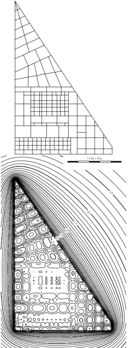
The first example is the E. R. Barber´a substation grounding (90×145m2) close to the city of Barcelona in Spain that is
operated by the power company FECSA. This earthing system (see figure 3) consist of 408 bars (φ= 12.85mm) buried to a depth of 80 cm.
Each conductor is discretized in one single linear density element (the aproximated leakage current density σh varies linearly within each conductor). This leads to an approximated problem with a total of 238 unknowns. Figure 3 shows the
Fig. 3. E.R. Barber´a substation grounding: Plan and potential distribution on the ground surface (contours plotted every 0.2 kV; thick contours every 1 kV).
computed potential distribution on the ground surface when a fault condition occurs. Figure 4 shows the computed potential profiles along two given lines on the ground surface. The computed Fault Current is IΓ = 31.8 kA, which gives an
Equivalent Resistance ofReq = 0.315 Ω.
This case was originally computed in a PC486/16Mb at 66MHz [12]. It took450 seconds to complete the analysis in 1997. The same analysis can be performed in about15seconds using a regular PC in 2002.
1 Unit = 10 m
150.
0.
0. 25. 50. 75. 100. 125. 150.
Distance (m)
0.0
2.0
4.0
6.0
8.0
10.0
Potential (kV)
1 Unit = 10 m 0.
175.
0. 25. 50. 75. 100. 125. 150. 175.
Distance (m)
0.0
2.0
4.0
6.0
8.0
10.0
Potential (kV)
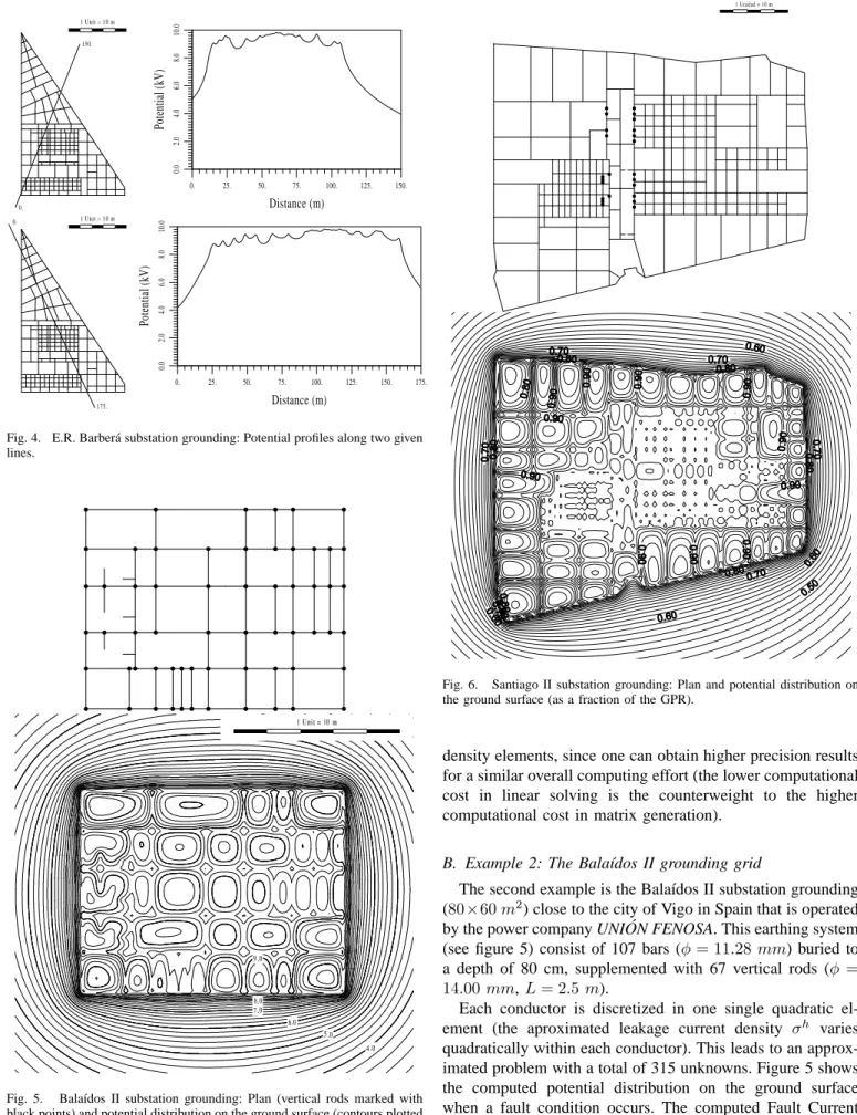
Fig. 4. E.R. Barber´a substation grounding: Potential profiles along two given lines.
Fig. 5. Bala´ıdos II substation grounding: Plan (vertical rods marked with black points) and potential distribution on the ground surface (contours plotted every 0.2 kV; thick contours every 1 kV).
Fig. 6. Santiago II substation grounding: Plan and potential distribution on the ground surface (as a fraction of the GPR).
density elements, since one can obtain higher precision results for a similar overall computing effort (the lower computational cost in linear solving is the counterweight to the higher computational cost in matrix generation).
B. Example 2: The Bala´ıdos II grounding grid
The second example is the Bala´ıdos II substation grounding (80×60m2) close to the city of Vigo in Spain that is operated
by the power company UNI ´ON FENOSA. This earthing system
(see figure 5) consist of 107 bars (φ= 11.28mm) buried to a depth of 80 cm, supplemented with 67 vertical rods (φ = 14.00mm,L= 2.5 m).
Each conductor is discretized in one single quadratic el-ement (the aproximated leakage current density σh varies quadratically within each conductor). This leads to an approx-imated problem with a total of 315 unknowns. Figure 5 shows the computed potential distribution on the ground surface when a fault condition occurs. The computed Fault Current was IΓ = 25.0 kA, which gives an Equivalent Resistance of
This case was also originally computed in a PC486/16Mb at 66MHz [12]. It took 600 seconds to complete the analysis in 1997. The same analysis can be performed in about 20 seconds using a regular PC in 2002.
In this case, using one single constant density element per conductor leads to an approximated problem with 174 un-knowns, while using one single linear density element per con-ductor leads to an approximated problem with 141 unknowns. This example shows that using quadratic density elements leads to larger approximated problems than using constant or linear density elements. Obviously, the computational cost devoted to matrix generation and linear solving is higher. However, the overall computing effort is still acceptable (in the same order of magnitude), while the precision of the results is much higher.
C. Example 3: The Santiago II grounding grid
The third (and final) example is the Santiago II substation grounding (230 ×195 m2) close to the city of Santiago
de Compostela in Spain that is also operated by the power company UNI ´ON FENOSA. This earthing system (see figure
6) consist of 534 bars (φ= 11.28mm) buried to a depth of 75 cm, supplemented with 24 vertical rods (φ= 15.00 mm, L= 4.0 m). The earth resistivity is 60 Ωm.
Each bar is discretized in one single linear density element, while each rod is discretized in two linear density elements. This leads to an approximated problem with a total of 386 unknowns. Figure 6 shows the computed potential distribution on the ground surface when a fault condition occurs. The computed Fault Current is IΓ = 67.3 kA, which gives an
Equivalent Resistance of Req= 0.149 Ω.
This case was originally computed in a DEC AlphaServer 4000–AXP running VMS [25], [26]. It took 7.7 seconds to complete the analysis in 1990. The same analysis can be performed in less than20seconds using a regular PC in 2002.
D. The effect of increasing the segmentation
The above mentioned examples have been repeatedly solved for an increasing segmentation of the electrodes. As the theory predicts (and it has been reported) the numerical instabilities pollute the results when the discretization is refined beyond a certain point.
Anyway, it seems that a reasonable (moderate) level of segmentation is sufficient to obtain quite accurate results in practice. In our experience, increasing the number of elements was needless in all the studied cases, since the results (at the scale of the whole grid) were not noticeably improved. It seems that increasing the segmentation is only justified when high accuracy local results are required for a limited part of the whole earthing system.
On the other hand, the use of higher order elements (liner or quadratic) seems to be more advantageous (in general) than increasing intensively the segmentation of constant elements, since the accuracy is higher for a remarkably smaller total number of degrees of freedom [11].
E. Further Developments
The techniques described in this paper can be extended for multi-layer soil models [25], [26], although computing time becomes not contemptible whatsoever. The proposed formulation has been implemented in a high-performance parallel computer and the code has been applied to the analysis of several real grounding systems [23], [25], [26]. The results obtained by the authors with the multi-layer code have been noticeably different from those obtained by using a single layer soil model. Thus, it is the authors’ belief that the proposed multi-layer BEM formulation will become a real-time design tool in a close future, as high-performance parallel computing becomes a widespread available resource in engineering. The formulation can also be adapted for computing transferred potentials [11].
VIII. CONCLUSIONS
A Boundary Element approach for the analysis of substation earthing systems has been presented. For 3D problems, some reasonable assumptions allow to reduce a general 2D BEM formulation to an approximated less expensive 1D version. Further simplifications reduce computing requirements under acceptable levels. Several widespread methods are identified as particular cases of this approach. In this theoretical framework, problems encountered with the application of these methods have been finally explained from a mathematically rigorous point of view. On the other hand, more efficient and accurate formulations have been derived. New analytical integration techniques allow to obtain accurate results in practical cases with acceptable computing requirements.
The techniques derived by the authors have been imple-mented in a Computer Aided Design system called TOTBEM. At present, this system runs in real-time in personal computers, and it has been used by the authors and by Spanish power com-panies to analyze several medium/large installations during the last 8 years. The techniques described in this paper have also been extended for multi-layer soil models and transferred potentials.
ACKNOWLEDGMENTS
This work has been partially supported by the Ministerio
de Educaci´on y Cultura of the Spanish Government (grant #
1FD97-0108 and # DPI2001-0556), cofinanced with European Union FEDER funds, by the power company Uni´on Fenosa
Ingenier´ıa S.A., and by research fellowships of the Xunta de Galicia and the Universidad de A Coru˜na.
APPENDIXI:
INTEGRALEXPRESSION FOR THEPOTENTIAL
We wish to obtain an integral expression for the solution V(xxx) to problem (1) at an arbitrary pointxxxxxxxxxxx xxxxxxxxxxxxxxinE. We assume that the earth surfaceΓE is horizontal.
ε x r ( x , )
Fig. 7. Extended symmetric domain for problem (1).
Ω(R). Let Γ0 be the image of the earthing electrode surface
Γ with respect to the plane ΓE. We assume that R is large enough. Thus, the earthing electrode and its symmetric are embedded —but not included— in Ω(R)(see figure 7).
The soil is considered homogeneous and isotropic. Thus, the tensorγγγγγγγγγγγγγγ is substituted by the constant scalar conductivity γ. In these terms, problem (1) can be substituted by the Dirichlet Exterior Problem
4V(zzzzzzzzzzzzzz) = 0 ∀zzzzzzzzzzzzzz∈Ω(∞),
V(ξξξξξξξξξξξξξξ) =VΓ ∀ξξξξξξξξξξξξξξ∈Γ, V(ξξξξξξξξξξξξξξ0) =VΓ ∀ξξξξξξξξξξξξξξ0 ∈Γ0,
V(zzzzzzzzzzzzzz) verifies normal conditions when |zzzzzzzzzzzzzz| → ∞, (33)
since the natural boundary condition σσσσσσσσσσσσσσtnnnnnnnnnnnnnn
E = 0 in ΓE is automatically fulfilled due to the symmetry of the extended domain. The so-called normal conditions at infinity can be mathematically expressed as [7], [8]
¯ [27] to the above stated problem is
Ψ(zzzzzzzzzzzzzz) = 1
Ψ(zzzzzzzzzzzzzz) verifies normal conditions when |zzzzzzzzzzzzzz| → ∞, (36)
being δ the Dirac’s delta distribution. Therefore, the funda-mental solution can be interpreted as the particular solution of the field equation for a punctual source of current at the given pointxxxxxxxxxxxxxx[27].
The Laplacian of the fundamental solution (35) is obviously singular at zzzzzzzzzzzzzz=xxxxxxxxxxxxxx, but it vanishes at any other point. In order to avoid the singularity we define the ball B(xx, ε)xxxxxxxxxxxx of radiusε centered at pointxxxxxxxxxxxxxx(see figure 7). LetΓB(xxxxxxxxxxxxxx,ε)be the boundary
of B(xxxxxxxxxxxxxx, ε).
We now consider the closed domain D(R, ε) = Ω(R)−
B(zzzzzzzzzzzzzz, ε). Obviously, bothV(zzzzzzzzzzzzzz)andΨ(zzzzzzzzzzzzzz)are functions of class C2 in D(R, ε). Therefore, we can apply the second Green’s
Identity [17], [11] to our problem, which gives
Z Z Z
zzzzzzzzzzzzzz∈D(R,ε)
³
V(zzzzzzzzzzzzzz)4Ψ(zzzzzzzzzzzzzz)−Ψ(zzzzzzzzzzzzzz)4V(zzzzzzzzzzzzzz)
´
nD is the corresponding normal exterior unit field.
Both functions V(zzzzzzzzzzzzzz) and Ψ(zzzzzzzzzzzzzz) are harmonic in D(R, ε), since (33) and (36) are satisfied and the singularity at zzzzzzzzzzzzzz = x
x has been isolated. Therefore, the left hand side of (37) vanishes, what gives
Finally, it is obvious that (38) holds for arbitrarily large values of Rand arbitrarily low values ofε. Therefore we can write
lim
boundary of D(R, ε) consists of the exterior boundaries of 1) the earthing electrode (Γ), 2) the image of the earthing electrode (Γ0), and 3) the ball that isolates the singularity
(ΓB(xxxxxxxxxxxxxx,ε)). Hence andV(zzzzzzzzzzzzzz) satisfies (33) and (34), we can prove that[11]
Therefore (40) reduces to
Finally, we can take advantage of the symmetry to write[10], [11], [12]
whereξξξξξξξξξξξξξξ0is the symmetric ofξξξξξξξξξξξξξξwith respect to the earth surface. The function σ(ξξξξξξξξξξξξξξ)in (46) is clearly identified as the leakage current density at an arbitrary pointξξξξξξξξξξξξξξon the earthing electrode Γ.
Under the above assumptions we can also prove that (45) holds on the earthing electrode surface. Thus, we still can say
V(χχχχχχχχχ) =χχχχχ 1 4πγ
Z Z
ξξξξξξξξξξξξξξ∈Γ
k(χχχ, ξξξξξξξξξξξξξξ)χχχχχχχχχχχ σ(ξξξξξξξξξξξξξξ)dΓ, ∀χχχχχχχχχχχχχχ∈Γ. (48)
This is neither obvious nor trivial, and the proof requires a special discussion[11]. In this case, kernel (47) becomes singular atξξξξξξξξξξξξξξ=χχχχχχχχχχχχχχ. Since (48) still makes sense in spite of the singularity, (47) is said to be a weakly singular kernel.
We notice that expression (45) always satisfies the field equation, the natural boundary condition and the normal conditions at infinity for problem (1). Therefore, the only thing that remains to be done in order to solve this problem is to fulfill the essential boundary condition V = VΓ in Γ. We
shall enforce this by means of (48). Therefore, our problem is reduced to finding the unknown leakage current density distributionσ(ξ)inΓ that verifies
VΓ= 1
4πγ
Z Z
ξξξξξξξξξξξξξξ∈Γ
k(χχχχ, ξξξξξξξξξξξξξξ)χχχχχχχχχχ σ(ξξξξξξξξξξξξξξ)dΓ, ∀χχχχχχχχχχχχχχ∈Γ. (49)
Once the leakage current density distribution is known, we shall be able to compute the potential at any point by means of expression (45).
REFERENCES
[1] J.G. Sverak, W.K. Dick, T.H. Dodds and R.H. Heppe, Safe Substation Grounding, IEEE Trans. on Power Apparatus and Systems, Part I: 100, 4281–4290, (1981); Part II: 101, 4006–4023, (1982).
[2] ANSI/IEEE Std.80, Guide for Safety in AC Substation Grounding, IEEE, New York, USA, (1986); and Draft Guide for Safety in AC Substation Grounding, IEEE, New York, USA, (1999).
[3] J.G. Sverak, Progress in Step and Touch Voltage Equations of ANSI/IEEE Std 80. Historical Perspective, IEEE Trans. on Power Delivery, 13, 762–767, (1998).
[4] R.J. Heppe, Computation of Potential at Surface Above an Energized Grid or Other Electrode, Allowing for Non-Uniform Current Distribu-tion, IEEE Trans. on Power Apparatus and Systems, 98, 1978–1988, (1979).
[5] D.L. Garrett and J.G. Pruitt, Problems Encountered With the Average Potential Method of Analyzing Substation Grounding Systems, IEEE Trans. on Power Apparatus and Systems, 104, 3586–3596, (1985). [6] B. Thapar, V. Gerez, A. Balakrishnan, D.A. Blank, Simplified Equations
for Mesh and Step Voltages in AC Substation, IEEE Trans. on Power Delivery, 6, 601–607, (1991).
[7] E. Durand, ´Electrostatique, Masson, Paris, France, (1966).
[8] O.D. Kellog, Foundations of Potential Theory, Springer-Verlag, Berlin, Germany, (1967).
[9] P.P. Silvester and R.L. Ferrari, Finite Elements for Electrical Engineers, Cambridge University Press, Cambridge, U.K., (1996).
[10] F. Navarrina, I. Colominas and M. Casteleiro, Analytical Integration Techniques for Earthing Grid Computation by BEM, In: H. Alder, J.C. Heinrich, S. Lavanchy, E. O˜nate, B. Su´arez (Eds.), Numerical Methods in Engineering and Applied Sciences, 1197–1206, CIMNE Pub., Barcelona, Spain, (1992).
[11] I. Colominas, A CAD System for Grounding Grids in Electrical Installations: A Numerical Approach Based on the Boundary Element Integral Method (in Spanish), Ph.D. Thesis, Universidad de A Coru˜na, Spain, (1995).
[12] I. Colominas, F. Navarrina and M. Casteleiro, A Boundary Element Nu-merical Approach for Grounding Grid Computation, Comput. Methods Appl. Mech. Engrg., 174, 73–90, (1999).
[13] F.P. Dawalibi, D. Mudhekar Optimum Design of Substation Grounding in a Two-Layer Earth Structure, IEEE Trans. on Power Apparatus and Systems, 94, 252–272, (1975).
[14] H.S. Lee, J.H. Kim, F.P. Dawalibi, J. Ma Efficient Ground Designs in Layered Soils, IEEE Trans. on Power Delivery, 13, 745–751, (1998). [15] E.D. Sunde, Earth Conduction Effects in Transmission Systems,
McMil-lan, New York, USA, (1968).
[16] F. Navarrina, L. Moreno, E. Bendito, A. Encinas, A. Ledesma and M. Casteleiro, Computer Aided Design of Grounding Grids: A Boundary Element Approach, In: M. Heili¨o (Ed.), Mathematics in Industry, 307– 314, Kluwer Academic Pub., Dordrecht, The Netherlands, (1991). [17] I. Stakgold, Boundary Value Problems of Mathematical Physics,
MacMillan Co., London, UK, (1970).
[18] I. Colominas, F. Navarrina and M. Casteleiro, A Validation of the Boundary Element Method for Grounding Grid Design and Compu-tation, In: H. Alder, J.C. Heinrich, S. Lavanchy, E. O˜nate, B. Su´arez (Eds.), Numerical Methods in Engineering and Applied Sciences, 1187–1196, CIMNE Pub., Barcelona, Spain, (1992).
[19] C. Johnson, Numerical Solution of Partial Differential Equations by the Finite Element Method, Cambridge Univ. Press, Cambridge, USA, (1987).
[20] T.J.R. Hughes, The Finite Element Method, Prentice Hall, New Jersey, USA, (1987).
[21] A.N. Kolmogorov and S.V. Fomin, Introductory Real Analysis, Dover Publications, New York, USA, (1975).
[22] G. Pini and G. Gambolati, Is a Simple Diagonal Scaling The Best Pre-conditioner For Conjugate Gradients on Supercomputers?, Advances on Water Resources, 13, 147–153, (1990).
[23] I. Colominas, F. Navarrina, G. Mosqueira, J.M. Eiroa and M. Casteleiro, Numerical Modelling of Grounding Systems in High-Performance Parallel Computers, In: C.A. Brebbia and H. Power (Eds.), Boundary Elements XXII, WIT Press, Southampton, UK, (2000).
[24] I. Colominas, F. Navarrina and M. Casteleiro, A Boundary Element Formulation for the Substation Grounding Design, Advances in Engi-neering Software, 30, 693–700, (1999).
[25] I. Colominas, J. G´omez Calvi˜no, F. Navarrina and M. Casteleiro, Computer Analysis of Earthing Systems in Horizontally or Vertically Layered Soils, Electric Power Systems Research, 59, 149–156, (2001). [26] I. Colominas, F. Navarrina and M. Casteleiro, A Numerical Formulation for Grounding Analysis in Stratified Soils, IEEE Trans. on Power Delivery, 17, 587–595, (2002).
Ferm´ın Navarrina Civil Engineer, M.Sc. (Univ. Polit´ecnica de Madrid, 1983), Ph.D. (Univ. Polit`ecnica de Catalunya, 1987). Professor of Applied Math at the Civil Engineering School of the Univ. of A Coru˜na. His research fields are related to the development of numerical methods for analysis and design optimization in engineering. He has directed and/or collaborated in a number of R&D projects and is the author of more than 50 papers published in scientific journals and books.
Ignasi Colominas Industrial Engineer, M.Sc. (Univ. Aut`onoma de Barcelona, 1990), Ph.D. (Univ. de A Coru˜na, 1995). Associate Professor of Applied Math at the Civil Engineering School of the Univ. of A Coru˜na. His main research areas are those related with computational mechanics in engineering applications. He currently leads a R&D project of the Spanish Government with european funds for the computational design of grounding systems of electrical substations. He is member of IEEE.