Mesoscale eddies in the Western Mediterranean Sea: characterization and understanding from satellite observations and model simulations
273
0
0
Texto completo
(2) 2.
(3) THÈSE Pour obtenir le grade de. DOCTEUR DE L’UNIVERSITÉ DE GRENOBLE préparée dans le cadre d’une cotutelle entre l’Université de Grenoble et l’Universitat de les Illes Balears Spécialité : Physique appliquée à l’ocean Arrêté ministériel : le 6 janvier 2005 -7 août 2006. Présentée par. Romain Escudier Thèse dirigée par Ananda Pascual codirigée par Pierre Brasseur préparée au sein de l’Institut Mediterrani d'Estudi s Avançats (IMEDEA) et du Laboratoire de Glaciologie et Géophysique de l’Environnement (LGGE) dans les Écoles Doctorales de Fí si ca de l’UIB et Terre-UniversEnvironnement de l’UdG. Tourbillons mésoéchelle dans la Méditerranée occidentale : charactérisation et compréhension à l’aide d’observations altimetriques et de simulations numériques Thèse soutenue publiquement le « date de soutenance », devant le jury composé de :. Damiá Gomis Professeur à l’UIB, Président. Dudley Chelton Professeur émérite à l’OSU, Rapporteur. Jordi Font Professeur à l’ICM, Rapporteur. Bernard Barnier Directeur de Recherche CNRS (LGGE), Examinateur. Lionel Renault Chercheur à UCLA, Examinateur. Ananda Pascual Asca so Chercheuse titulaire CSIC (IMEDEA), Directrice de thèse Pierre Brasseur Directeur de Recherche CNRS (LGGE), Co-Directeur de thèse Université Joseph Fourier / Université Pierre Mendès France / Université Stendhal / Université de Savoie / Grenob le INP.
(4) 4.
(5) Acknowledgements Mes remerciements vont tout d’abord à Ananda Pascual pour m’avoir donné l’opportunité de réaliser cette thèse et son soutien tout au long de ces quatres années. Toujours à l’écoute, elle su me guider tout en sachant me laisser prendre des initiatives. Je voudrais ensuite remercier Pierre Brasseur pour avoir accepté de nous accompagner dans cette aventure. Encadrer la thèse à distance n’a pas toujours été facile mais Pierre a été là pour m’aider à prendre du recul voire réorienter mes recherches quand il le fallait. Je suis reconnaissant au CSIC qui, avec la bourse de thèse JAE, m’a permis de travailler sur ce sujet de thèse. Je remercie également le CNRS pour m’avoir financé mes derniers mois de thèse ainsi que le projet MyOcean2 qui m’a permis d’assister à plusieurs conférences au cours de ma thèse. Merci à Lionel Renault, qui m’a initié aux mystères de la modélisation. Même après s’être expatrié à l’autre bout du monde, il a continué à s’investir dans mon projet de thèse. Je souhaite également remercier Dudley Chelton pour son accueil à Corvallis, sa disponibilité et son apport scientifique. Un grand merci à tous ceux que j’ai rencontré au cours de cette thèse et qui ont fait de ces années une belle histoire. Je pense bien sûr aux collèques de l’IMEDEA (et SOCIB), qui, pour la plupart, sont devenus des amis. J’ai adoré nos discussions interminables, qu’elles aient été lors des séminaires ”imedeicos”, sur la terrasse à midi ou le soir autour d’une caña. Je pense aussi à toute l’équipe MEOM à Grenoble qui m’a fait sentir chez moi à chacun de mes séjours là-bas. L’ambiance chaleureuse et l’esprit d’entraide est une des grandes qualités de cette équipe. Je n’oublie pas les amis, à Palma, en France ou dispersé dans le monde, ainsi que ma famille qui ont souvent été le soutien dont j’avais besoin pour continuer. Merci à plus particulièrement à mes parents pour leurs conseils, leur soutien et leur aide dans la correction de ce manuscrit. i.
(6) ii Thank you all..
(7) Abstract Mesoscale eddies are relatively small structures that dominate the ocean variability and have large impact on large scale circulation, heat fluxes and biological processes. In the western Mediterranean Sea, a high number of eddies has been observed and studied in the past with in-situ observations. Yet, a systematic characterization of these eddies is still lacking due to the small scales involved in these processes in this region where the Rossby deformation radius that characterizes the horizontal scales of the eddies is small (10-15 km). The objective of this thesis is to perform a characterization of mesoscale eddies in the western Mediterranean. For this purpose, we propose to develop tools to study the fine scales of the basin. First, we develop an eddy resolving simulation of the region for the last 20 years. The performance of the simulation is evaluated with independent observations (drifters, satellites, hydrographic profiles) showing realistic behavior. This simulation shows that existing altimetry maps underestimate the mesoscale signal. Therefore, we attempt to improve existing satellite altimetry products to better resolve mesoscale eddies. We show that this improvement is possible but at the cost of the homogeneity of the fields; the resolution can only be improved at times and locations where altimetric observations are densely distributed. In a second part, we apply three different eddy detection and tracking methods to extract eddy characteristics from the outputs of the highresolution simulation, a coarser simulation and altimetry maps. The results allow the determination of some characteristics of the detected eddies. The size of the eddies can greatly vary but is around 25-30 km. About 30 eddies are detected per day in the region with a very heterogeneous spatial distribution. Unlike other areas of the open ocean, they are mainly advected by currents of the region. Eddies can be separated according to their lifespan. Long-lived eddies are larger in amplitude and scale and have a seasonal cycle iii.
(8) iv with a peak in late summer, while short-lived eddies are smaller and more present in winter. The penetration depth of detected eddies has also a large variance but the mean depth is around 300 meters. Anticyclones extend deeper in the water column and have a more conic shape than cyclones..
(9) Resumen Los remolinos de mesoescala son estructuras relativamente pequeñas que dominan la variabilidad del océano y tienen un fuerte impacto en la circulación de gran escala, los flujos de calor y los procesos biológicos. En el Mediterráneo occidental, se han estudiado numerosos remolinos a partir de observaciones in-situ. Sin embargo, todavı́a falta una caracterización sistemática de estos remolinos ya que las escalas implicadas en los procesos de esta región son pequeñas. Se estima que el radio de deformación de Rossby asociado a las escalas horizontales tı́picas de los remolinos varia entre 10 y 15 km. El objetivo de esta tesis es realizar una caracterización de los remolinos de mesoescala en el Mediterráneo occidental. Con este fin, se propone el desarrollo de herramientas para el estudio de las estas estructuras. En primer lugar, se implementa una simulación numérica de la región durante los últimos 20 años con una resolución suficiente para resolver remolinos. Usando observaciones independientes (boyas, satélites, perfiles hydrograficos) se demuestra el realismo de la simulación. Además esta simulación muestra que los mapas de altimetrı́a existentes subestiman la señal de la mesoescala. En este contexto, se propone un nuevo método para mejorar la resolución de los productos de altimetrı́a por satélite existentes con el objectivo de estudiar los remolinos de mesoescala. Se demuestra que el nuevo método mejora los mapas altimétricos, sin embargo, conlleva una pérdida de la homogeneidad de los campos; la resolución sólo puede mejorarse en determinados momentos y lugares en los que las observaciones altimétricas están presentes de forma muy densa. En la segunda parte de la tesis, se aplican tres métodos diferentes de detección y de seguimiento de remolinos para extraer las caracterı́sticas de los remolinos a partir de las salidas tanto de la simulación de alta resolución, como de una simulación más de menor resolución y de los mapas de altimetrı́a. Los resultados permiten determinar algunas propriedades de los v.
(10) vi remolinos detectados. El radio de los remolinos puede variar mucho pero la mayorı́a es alrededor de 25-30 km. Aproximadamente se detectan 30 remolinos por dı́a en la región con una distribución espacial muy heterogénea. A diferencia de otras zonas del océano abierto, éstos son principalmente advectados por las corrientes de la región. Podemos separar los remolinos según su tiempo de vida. Los remolinos de vida larga (más de cuatro semanas) tienen mayor amplitud y escala y tienen un ciclo estacional con un pico a finales de verano, mientras que los remolinos de corta duración son más pequeños y más presentes en invierno. La profundidad de penetración de los remolinos detectados tiene también una gran variabilidad con un valor medio de alrededor 300 m. Los remolinos anticiclónicos se extienden más profundamente en la columna de agua y muestran una forma más cónica que los ciclónicos..
(11) Contents Page Aknowledgements. iii. Abstract. v. Resumen. vii. Contents. vii. 1 Motivation and objectives. 1. 2 The Western Mediterranean Sea. 9. 2.1. Geography . . . . . . . . . . . . . . . . . . . . . . . . . . . .. 10. 2.2. Forcings . . . . . . . . . . . . . . . . . . . . . . . . . . . . .. 11. 2.3. General circulation and water masses . . . . . . . . . . . . .. 13. 2.3.1. Surface circulation . . . . . . . . . . . . . . . . . . .. 13. 2.3.2. Water masses . . . . . . . . . . . . . . . . . . . . . .. 15. Mesoscale dynamics . . . . . . . . . . . . . . . . . . . . . . .. 16. 2.4.1. Alboran Sea . . . . . . . . . . . . . . . . . . . . . . .. 16. 2.4.2. Algerian Basin . . . . . . . . . . . . . . . . . . . . .. 17. 2.4.3. Algero-Provençal basin . . . . . . . . . . . . . . . . .. 18. 2.4.4. Liguro-Provençal basin and Gulf of Lion . . . . . . .. 19. 2.4.5. Balearic Sea . . . . . . . . . . . . . . . . . . . . . . .. 20. Recent advances in modelling and global observations of the mesoscale in the WMED . . . . . . . . . . . . . . . . . . . .. 21. 2.5.1. Observing systems . . . . . . . . . . . . . . . . . . .. 21. 2.5.2. Altimetry . . . . . . . . . . . . . . . . . . . . . . . .. 24. 2.5.3. Modelling . . . . . . . . . . . . . . . . . . . . . . . .. 29. 2.4. 2.5. vii.
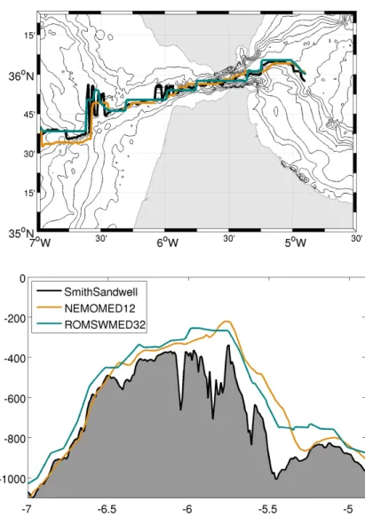
(12) viii 3 A high resolution model of the area 3.1 Objective . . . . . . . . . . . . . . . . . . 3.2 ROMS model . . . . . . . . . . . . . . . . 3.2.1 Primitive equations . . . . . . . . . 3.2.2 Vertical boundary conditions . . . . 3.2.3 Terrain-following coordinate system 3.3 Physical parameterizations . . . . . . . . . 3.3.1 Advection schemes . . . . . . . . . 3.3.2 Boundary layer parameterization . 3.4 Spatial and temporal discretization . . . . 3.5 Topography . . . . . . . . . . . . . . . . . 3.5.1 Pressure gradient error . . . . . . . 3.5.2 Gibraltar . . . . . . . . . . . . . . 3.6 Initial state and boundary conditions . . . 3.6.1 NEMOMED12 simulation . . . . . 3.6.2 Initial conditions . . . . . . . . . . 3.6.3 Boundary parameterization . . . . 3.7 Atmospheric forcings . . . . . . . . . . . . 3.7.1 Flux forcing . . . . . . . . . . . . . 3.7.2 Bulk parameterization . . . . . . . 3.8 Rivers . . . . . . . . . . . . . . . . . . . . 3.9 Set of simulations . . . . . . . . . . . . . . 3.10 Computing resources . . . . . . . . . . . . 3.11 Conclusion . . . . . . . . . . . . . . . . . .. CONTENTS. . . . . . . . . . . . . . . . . . . . . . . .. . . . . . . . . . . . . . . . . . . . . . . .. . . . . . . . . . . . . . . . . . . . . . . .. . . . . . . . . . . . . . . . . . . . . . . .. . . . . . . . . . . . . . . . . . . . . . . .. 4 Analysis and validation of a 20-years simulation resolution 4.1 Objective . . . . . . . . . . . . . . . . . . . . . . . 4.2 Observational products used for the validation . . . 4.2.1 Altimetry . . . . . . . . . . . . . . . . . . . 4.2.2 SST . . . . . . . . . . . . . . . . . . . . . . 4.2.3 Temperature and salinity fields . . . . . . . 4.2.4 Drifters . . . . . . . . . . . . . . . . . . . . 4.3 Surface circulation . . . . . . . . . . . . . . . . . . 4.3.1 Mean circulation . . . . . . . . . . . . . . . 4.3.2 Focus on the Alboran Sea . . . . . . . . . . 4.4 Surface variables . . . . . . . . . . . . . . . . . . .. . . . . . . . . . . . . . . . . . . . . . . .. . . . . . . . . . . . . . . . . . . . . . . .. . . . . . . . . . . . . . . . . . . . . . . .. . . . . . . . . . . . . . . . . . . . . . . .. . . . . . . . . . . . . . . . . . . . . . . .. 33 34 35 35 36 37 40 40 40 41 42 42 45 47 47 48 48 49 49 50 50 51 51 54. at 1/32◦ . . . . . . . . . .. . . . . . . . . . .. . . . . . . . . . .. . . . . . . . . . .. . . . . . . . . . .. 59 60 60 61 62 62 63 64 64 66 70.
(13) CONTENTS 4.4.1 Sea Surface Temperature 4.4.2 Sea Surface Salinity . . . 4.5 Under the surface . . . . . . . . 4.5.1 Heat and salt content . . 4.5.2 Water masses . . . . . . 4.6 Deep water convection . . . . . 4.7 Transports . . . . . . . . . . . . 4.7.1 Time evolution . . . . . 4.7.2 Velocity section . . . . . 4.8 Spectra . . . . . . . . . . . . . 4.9 EKE . . . . . . . . . . . . . . . 4.10 Eddy heat transport . . . . . . 4.11 Conclusion . . . . . . . . . . . .. ix . . . . . . . . . . . . .. . . . . . . . . . . . . .. . . . . . . . . . . . . .. . . . . . . . . . . . . .. . . . . . . . . . . . . .. . . . . . . . . . . . . .. . . . . . . . . . . . . .. . . . . . . . . . . . . .. . . . . . . . . . . . . .. . . . . . . . . . . . . .. . . . . . . . . . . . . .. . . . . . . . . . . . . .. . . . . . . . . . . . . .. . . . . . . . . . . . . .. . . . . . . . . . . . . .. . . . . . . . . . . . . .. 70 70 74 74 79 82 85 85 85 88 89 91 94. 5 One step towards better observational data: High resolution altimetry 95 5.1 Objective . . . . . . . . . . . . . . . . . . . . . . . . . . . . 97 5.2 Escudier et al. 2013 . . . . . . . . . . . . . . . . . . . . . . . 97 5.3 Auxiliary material . . . . . . . . . . . . . . . . . . . . . . . 104 5.3.1 Rossby radius . . . . . . . . . . . . . . . . . . . . . . 104 5.3.2 Supplementary figures . . . . . . . . . . . . . . . . . 104 5.4 Conclusions and perspectives . . . . . . . . . . . . . . . . . . 108 6 Eddy detection and tracking 6.1 Objective . . . . . . . . . . . . . . . . . . . . . . . 6.2 Methods and data . . . . . . . . . . . . . . . . . . . 6.2.1 Detection method: Closed contours of SLA . 6.2.2 Other methods . . . . . . . . . . . . . . . . 6.2.3 Datasets . . . . . . . . . . . . . . . . . . . . 6.3 Results . . . . . . . . . . . . . . . . . . . . . . . . . 6.3.1 Preliminary study on satellite altimetry . . . 6.3.2 Application to simulations . . . . . . . . . . 6.3.3 Application to the high resolution altimetry 6.4 Conclusion . . . . . . . . . . . . . . . . . . . . . . .. . . . . . . . . . .. . . . . . . . . . .. . . . . . . . . . .. . . . . . . . . . .. . . . . . . . . . .. 111 113 114 114 119 123 124 124 133 162 167. 7 Conclusions and perspectives 169 7.1 Conclusions . . . . . . . . . . . . . . . . . . . . . . . . . . . 169 7.2 Perspectives . . . . . . . . . . . . . . . . . . . . . . . . . . . 171.
(14) x. CONTENTS. List of Figures. 173. List of Tables. 177. Bibliography. 179. Appendices. 203. A Bouffard et al. 2014. 203. B Gomez Enri et al. 2014. 219. C Optimal interpolation 249 C.1 Theory . . . . . . . . . . . . . . . . . . . . . . . . . . . . . . 249 C.2 Application . . . . . . . . . . . . . . . . . . . . . . . . . . . 252 C.3 Method in two steps . . . . . . . . . . . . . . . . . . . . . . 253.
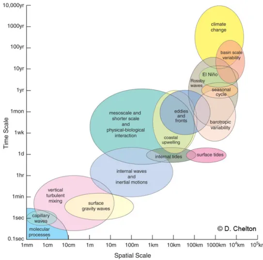
(15) Chapter 1 Motivation and objectives Motivation While appearing stable, the ocean is in fact an agitated fluid that never stops moving. These motions cover a wide range of spatial and temporal scales as illustrated in figure 1.1. In this figure, processes with a spatial scale from 1 mm to 105 km and temporal scales from 0.1 seconds to 10000 years are identified. In physical oceanography, these scales are usually separated into three categories. Large scales or synoptic scales represent the mean currents and permanent structures as well as very large (more than 500 km) and slow processes (more than 100 days). Mesoscale dynamics which dominate the variability of the ocean (Chelton et al., 2007), cover transient coherent structures that are smaller and faster than large scale structures. Finally, sub-mesoscale processes are smaller than the mesoscale and can be caused by mesoscale dynamics through frontogenesis or created by ageostrophic baroclinic instabilities (e.g. Molemaker et al. 2005) as well as forced motions due to atmospheric forcing (Thomas et al., 2008). The focus of this thesis is the mesoscale structures which are omnipresent at global ocean and play a key role in multiple ocean processes but are not yet fully analyzed and monitored in a global scale due to their relatively small size. A useful dimensionless number which enables us to separate the mesoscale from the submesoscale, based on their dynamical properties is the Rossby number (Ro). This number is the ratio between inertial force and the Coriolis acceleration force due to the rotation of the Earth in the Navier-Stokes equations. U Ro = (1.1) Lf 1.
(16) 2. Figure 1.1: Scales of the main processes in the ocean. Courtesy of D. Chelton.. where U is a characteristic velocity, L a characteristic length scale and f is the Coriolis frequency i.e. f = 2Ω sin(Φ) with Ω the rotational speed of the Earth and Φ the latitude. If this number is large (high speed or small size), inertial and centrifugal forces dominate and Coriolis forces can be neglected at the first order. If conversely, it is small, it means that the fluid is significantly affected by rotational effects and these must be included in the computations of the flow. In this case, an equilibrium is found between Coriolis forces and the pressure gradient of the fluid, and this state is called geostrophic balance. Mesoscale processes have small Rossby number (O(0.1)) and are sometimes called quasi-geostrophic motions as you can apply the geostrophic balance to them. This means the geostrophic.
(17) CHAPTER 1. MOTIVATION AND OBJECTIVES. 3. currents (ug , vg ) can be computed from the pressure (p) gradient as: 1 ∂p ρ ∂x 1 ∂p f ug = − ρ ∂y f vg =. (1.2). Sub-mesoscale processes which have a Rossby number (O(1)) cannot be described by quasi-geostrophic theory and therefore have to be separated from mesoscale processes (Thomas et al., 2008). The Rossby number is associated with the Rossby radius of deformation, the length scale at which Coriolis forces become as important as inertial forces. An estimation of this scale is (Chelton et al., 1998): Z 0 1 N (z) dz (1.3) Rd = |f |π −H with N (z) the BruntVaisala frequency and H the scale height. This scale gives us the lower limit for the mesoscale structures in terms of size. The corresponding upper limit cannot be so easily defined and is usually defined to be smaller than the scale of the main currents. In this thesis and in our region of study, the upper limit will not be defined in term of size but in term of temporal duration. Indeed, we define mesoscale processes as transient processes which separate them from the main circulation. We will see that, with our detection algorithms, it correspond to the size that is generally arbitrarily defined as the definition of mesoscale in the Mediterranean Sea. Although mesoscale phenomena can take various forms such as vortices, meanders, rings or narrow jets, they are mainly composed of eddies. Ocean mesoscale eddies, which are at the core of the thesis, can be defined as oceanic currents flowing in a relatively circular pattern. Mesoscale eddies are stable due to geostrophic balance such that gravitational forces are compensated by Coriolis forces. Mesoscale eddies are ubiquitous in the ocean as observed by satellite altimeters in Chelton et al. (2007) with energy levels usually above those of the mean flow by one or more orders of magnitude. These estimations come from current velocities calculated from merchant ships (Wyrtki et al., 1976), surface drifters (Richardson, 1983) or altimetry and numerical models (Thoppil et al., 2011). High levels of Eddy Kinetic Energy (EKE), the transient part of the Kinetic Energy (KE), are found along the main fronts in the ocean (Western boundary currents such as the Gulf Stream and Kuroshio Current.
(18) 4 or the Brazil-Malvinas Confluence) as shown by Ducet et al. (2000), indicating that the most frequent mechanism for the formation of these structure can be baroclinic instability of the mean currents. This instability occurs in strongly stratified fluids where there is a vertical shear of the horizontal velocity. In these cases, the fluid can be stable (geostrophic equilibrium) but not at the lowest energy level possible and therefore, there is a supply of available potential energy. Under certain conditions, an instability can form and there is a transfer of this potential energy to the kinetic energy of the disturbance, thereby boosting its growth. Another possible instability is barotropic instability which occurs when there is a strong horizontal shear of the current. In this case, the transfer of energy is between kinetic energy of the mean flow and kinetic energy of the instability. Oceanic mean flows have both vertical and horizontal shears which means that both instabilities can coexist. In regions where there is no strong mean current, mesoscale eddies can be directly generated by the fluctuating wind (Frankignoul and Müller, 1979). Willett et al. (2006) have also proposed that the coastal eddies in the coastal region between southern Mexico and Panama are created by Ekman pumping associated with the wind stress curl. Finally, interactions of currents with topography can be a potential mechanism for the generation of mesoscale eddies. This is apparent in EKE maps where high energy is found near major topographic obstacles. Because of their non-linear dynamics, eddies transport water mass with its heat content as well as chemical (e.g. salt) and biological properties (e.g. nutrients, biomass) over large distances (McWilliams, 1985). Their crucial role in the transport of heat fluxes has been shown in many studies (Wunsch, 1999; Jayne and Marotzke, 2002; Colas et al., 2012) but the relevance of eddy transport in the Mediterranean is still unknown. Eddy salt transport (Zhurbas et al., 2004) could be significant in the Mediterranean since its density structure is mainly driven by salinity. Concerning biology, apart from transporting biomass (Feng et al., 2007; Llinás et al., 2008), mesoscale eddies modify the local Mixed Layer Depth (MLD), significantly enhancing primary production (Oschlies and Garçon, 1998; Levy et al., 1998; Mahadevan et al., 2012). Mesoscale eddies can also feed energy back to the main flow and drive large scale circulation (Lozier, 1997; Holland, 1978), making them a key component of the ocean dynamics. In this thesis, the purpose is to study mesoscale dynamics in a challeng-.
(19) CHAPTER 1. MOTIVATION AND OBJECTIVES. 5. ing region: the Western Mediterranean Sea (WMed). In this semi-enclosed basin, the Rossby deformation radius is relatively small: 10-15 km (Robinson et al., 2001) and therefore mesoscale structures vary in size from 10-15 km to 150 km. As explained above, the upper limit here is the one usually given but was also confirmed by our analysis of mesoscales defined as non permanent structures. Figure 1.2 (extracted from Beuvier et al. 2012) shows the Rossby radius (Ro) that is computed from the MEDATLAS database (MEDAR Group et al., 2003) following the equation 1.3. In the WMed, we see that Ro ranges from 6 km at the south-eastern coast of France to 15 km north of the Algerian shore. Over shallow shelves such as in the Gulf of Lion, it is even smaller at around 3 km.. Figure 1.2: First Rossby radius of deformation (km, contours every 5 km), computed from the MEDATLAS database state representative of the end of the 1990s and from the bathymetry of NEMOMED12. Figure extracted from Beuvier et al. (2012).. Objective This small Rossby radius has prevented a systematic monitoring of mesoscale activity in the WMed region. Indeed, sparse in situ data or crude model simulations have not been enough to obtain a statistical robust and homogeneous picture of mesoscale activity. Therefore there are still some crucial scientific issues associated with WMed eddies. First, there is the characterization of mesoscale activity in.
(20) 6 the region. What are its magnitude, its spatial patterns and temporal variability? How are these mesoscale structures in terms of size, intensity and anomalies in density which they provoke? Then questions about the formation of these mesoscale eddies in the WMed are still unanswered and work is still needed to understand the role of wind, topography or instabilities of currents. Finally, we lack an evaluation on the impact of mesoscale activity on large scale processes, heat and salt fluxes, and biological mechanisms. All these question are inter-connected and are critical if we want to predict the evolution of mesoscale processes and their impact on ecosystems. Some of these questions have been answered in part by the community using the available tools in terms of observation and numerical modelling which we describe in chapter 2. Yet, these tools are not enough to fully understand mesoscale in the Western Mediterranean and to try and begin to answer some of these questions, we will develop new tools to study the mesoscale in the WMed. These new tools will need datasets with resolution high enough to monitor mesoscale eddies in the region. The increasing computing power available for numerical modelling enables the design of continuously higher resolution simulations that can now approach the full resolution of mesoscale dynamics. Therefore, new high resolution, long-term, simulation of the WMed that is eddy-resolving is developed toward this specific goal. Its implementation is described in chapter 3 and its outputs are analyzed and validated in chapter 4, with the objective of representing mesoscale activity in the region of study well. High resolution observational data is an excellent complementary source of information that can be used in combination with the model outputs. In this idea, we attempt to improve existing satellite altimetry gridded maps which now cover a relatively long period of time (1992-2012) with the focus on better resolving mesoscale dynamics in chapter 5. Then, automatic eddy detection and tracking algorithms of eddies helps us to characterize mesoscale eddies in the region. These algorithms are applied on satellite altimetry maps, the high resolution model and a lower resolution model outputs in chapter 6. These tools allow us to shed some light on the characterization of the mesoscale dynamic, the first scientific issue stressed above. The spatial and temporal distribution of mesoscale eddies is determined as well as physical characteristics of the eddies. Some hypotheses on the formation processes and the influence of wind are examined but more study is required and the tools we develop will help in this endeavor. The impact of mesoscale activity is studied with the.
(21) CHAPTER 1. MOTIVATION AND OBJECTIVES help of the models but the issue is still a work in progress.. 7.
(22) 8.
(23) Chapter 2 The Western Mediterranean Sea Contents 2.1. Geography. . . . . . . . . . . . . . . . . . . . . . .. 10. 2.2. Forcings . . . . . . . . . . . . . . . . . . . . . . . .. 11. 2.3. General circulation and water masses . . . . . .. 13. 2.4. 2.5. 2.3.1. Surface circulation . . . . . . . . . . . . . . . . .. 13. 2.3.2. Water masses . . . . . . . . . . . . . . . . . . . .. 15. Mesoscale dynamics . . . . . . . . . . . . . . . . .. 16. 2.4.1. Alboran Sea . . . . . . . . . . . . . . . . . . . . .. 16. 2.4.2. Algerian Basin . . . . . . . . . . . . . . . . . . .. 17. 2.4.3. Algero-Provençal basin . . . . . . . . . . . . . . .. 18. 2.4.4. Liguro-Provençal basin and Gulf of Lion . . . . .. 19. 2.4.5. Balearic Sea . . . . . . . . . . . . . . . . . . . . .. 20. Recent advances in modelling and global observations of the mesoscale in the WMED . . . . .. 21. 2.5.1. Observing systems . . . . . . . . . . . . . . . . .. 21. 2.5.2. Altimetry . . . . . . . . . . . . . . . . . . . . . .. 24. 2.5.3. Modelling . . . . . . . . . . . . . . . . . . . . . .. 29. 9.
(24) 10. 2.1. GEOGRAPHY. The Mediterranean Sea is a relatively small sea but with huge importance because of several factors. First, it is the birthplace of several major civilizations and thus people started studying it a long time ago. During a very long period of time, the Mediterranean was the main mean of transport for goods and people in the region. It is now suffering strong anthropogenic pressure due to the density of human population living along its coasts and it is crucial to study and understand the impacts of this pressure (Hulme et al., 1999). What also makes the Mediterranean Sea unique and valuable for scientists is that many fundamental processes that occur in the global ocean happen there at a smaller scale. That is why it is often called a miniature ocean (Bethoux et al., 1999). The dimensions and mid-latitude location of the Mediterranean makes it easier to study and sample. Examples of such processes are deep convection (Herrmann and Somot, 2008), cascading, thermohaline circulation and water mass interactions (Wüst, 1961), baroclinic instabilities (Millot, 1987), transport through small straits and mesoscale activity (Robinson et al., 2001). Finally, the Mediterranean Sea is a concentration basin, as there is more evaporation than precipitation at the surface. Therefore, there is a formation of salty water called Mediterranean Water (MW) that enters the Atlantic, participates in the circulation of this ocean and consequently impact on the global thermohaline conveyor belt (Broecker et al., 1991). Potter and Lozier (2004) reported the impact of the warmed up MW on the Atlantic heat content and therefore on the climate at mid-latitudes. The MW then propagates far north until the Norwegian-Greenland Sea as described by Arhan (1987) where it can influence the deep water formation (Schmitz Jr, 1996; Iorga and Lozier, 1999) or directly impacts them on their return circulation as proposed by Keeling and Peng (1995).. 2.1. Geography. The Mediterranean Sea is an almost enclosed sea between 5◦ W and 36◦ E in longitude and 30◦ N and 46◦ N in latitude with a total area of 3,000,000 km2 . It separates Europe from the African continent. The narrow (22 km) and shallow (300 m) Gibraltar Strait at the south of Spain connects the Sea with the Atlantic Ocean. The Mediterranean Sea is composed of two main basins linked by the Sicilian Strait: the Eastern.
(25) CHAPTER 2. THE WESTERN MEDITERRANEAN SEA. 11. Figure 2.1: An overview of the Western Mediterranean. Basin and the Western Basin. The Western basin (hereafter WMed) which is the focus of this thesis is shown on figure 2.1. It is composed of various sub-basins : the Alboran Sea, the Algerian basin, the Balearic Sea, the Liguro-Provencal basin and the Tyrrhenian Sea. As shown on the figure, the topography is rugged and the coastlines are jagged. To study the WMed, it is useful to separate the basin into different regions according to their general circulation patterns. Figure 2.2 shows these regions defined by Manca et al. (2004) that we will use in this thesis.. 2.2. Forcings. The Gibraltar Strait forcing is crucial to the Western Mediterranean circulation as it is the source of fresh water that will feed the entire Mediterranean thermohaline circulation. The transport through the strait has three components: a tidal induced barotropic one with velocities of about 2.5 m.s-1 and two baroclinic components. The first baroclinic component is due to atmospheric difference of pressure over the Mediterranean (Gomis et al., 2006) creating velocities of about 0.4 m.s-1 (Candela et al., 1989) and the second one, the long-term component is driven by the water budget of the Mediterranean which is a concentration basin and thus needs some input from the Atlantic, inducing velocities of about 0.5 m.s-1 . Astraldi et al. (1999) made a review on the estimated transport through the strait from observation up to 1999 but the estimates vary greatly depending on the method used to compute it. The methods can be direct measurements or.
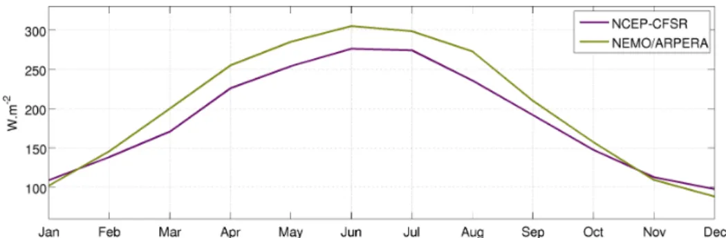
(26) 12. 2.2. FORCINGS. indirect computations by the Mediterranean budget, hydrodynamic properties of the strait or computation of geostrophic balance. The uncertainty about these estimates also comes from the fact that most of them are computed from short data series (less than 1 year) or have strong assumptions. Estimates of the Atlantic inflow range between 0.72 and 1.60 Sv (1 Sv = 106 m3 .s-1 ), the outflow ranges between 0.80 and 1.68 Sv and the net exchange is of the order of tenths of Sv. More recently, using in-situ observations Soto-Navarro et al. (2010) measured the outflow at -0.78 ± 0.05 Sv and the resulting inflow at 0.81 ± 0.06 while Criado-Aldeanueva et al. (2012) estimated the inflow to be around 0.82 ± 0.05 Sv. The transport in the Gibraltar Strait has also been studied using numerical models such as the work by Beranger et al. (2005) or Sannino et al. (2009). The high mountain chains around the basin (Pyrenees, Alps, Atlas) constrain the lower atmospheric layer and create very strong local winds that flow over the Mediterranean. These winds, in the western part of the basin, can come from the north such as the Tramontane, Mistral and Bora, or from the south such as the Sirocco (figure 2.1). The circulation in the Mediterranean Sea is strongly constricted by these local winds but interconnections with large scale atmospheric forcings have been found (Xoplaki et al., 2004; Josey et al., 2011). Northerly winds bring cold and dry air above the sea, causing strong evaporation and therefore latent heat loss. This effect is the dominant one in the Mediterranean whose net water and heat flux is negative. This loss is compensated at the Gibraltar Strait by the water and heat transport described above where a little warmer and fresh Atlantic waters enter the Mediterranean Sea. With in-situ observations from moored instruments Macdonald et al. (1994) estimated the heat transport into the Mediterranean through the strait at 5.2 ± 1.3W.m2 . Other authors gave estimations ranging from 5 W.m2 (Bunker et al., 1982) to 8.5 W.m2 (Bethoux, 1979). A more complete budget of the area with more that 40 years of reanalysis is given by Ruiz et al. (2008). They confirmed the importance of latent heat in the budget and gave new estimates of the different terms. In the Western Mediterranean, they show that the heat budget is actually positive which means a heating of the Sea with a value of 5 W.m2 in the basin whereas the whole basin has a net heat flux of -1 W.m2 . Estimation of the loss of water is more uncertain due to the difficulties to have good estimates of the evaporation and precipitation fluxes. (Bethoux,.
(27) CHAPTER 2. THE WESTERN MEDITERRANEAN SEA. 13. 1979) gives a value of -0.95 m.year-1 on the surface of the Mediterranean Sea (2.5 1012 m2 ). Since then many authors have taken on the task of estimating these fluxes for the whole Mediterranean basin, Bryden et al. (1994) made a review of these estimates ranging between 0.47 m.year-1 and 1.31 m.year-1 . This water loss is compensated by the net water coming into the Mediterranean at the Gibraltar Strait. Another external influence on the Mediterranean Sea is river inflow. In the WMed, the main rivers are the Rhône (mean discharge : 1710 m3 .s-1 ) and the Ebro river (mean discharge : 426 m3 .s-1 ). These discharges are not trivial as the Rhône, for example, injects the equivalent of 0.02 m of water to the surface of the whole Mediterranean Sea per year (Tomczak and Godfrey, 2001). This is to be compared to precipitation values of around 0.34 m.year-1 and E-P-R around -1 m.year-1 . Bethoux and Gentili (1999) also show that Mediterranean rivers could play an important role in climate by studying the trends in salinity and temperature in the basin and linking these trends to changes in the river inflow.. 2.3 2.3.1. General circulation and water masses Surface circulation. The general surface circulation of the Western basin is mainly driven by the wind forcing in Sverdrup balance (Pinardi and Navarra, 1993; Molcard et al., 2002). This is shown in figure 2.1 and has been described by Millot (1999). Entering the WMed from the Gibraltar Strait to compensate the deficit of water due to the wind-induced high evaporation, fresh Atlantic Water (AW)1 forms the Atlantic jet. This strong current meanders through the Alboran gyres, the quasi permanent Western Alboran Gyre (WAG) and the intermittent Eastern Alboran Gyre (EAG). It then becomes the relatively narrow Algerian Current, flowing along the coast at first but becoming less clearly defined nor narrow as it progresses eastward. This is due to baroclinic instabilities that cause meanders and, eventually, eddies that detach from the main current (Olita et al., 2011). In the Tyrrhenian Basin, west of Corsica and Sardinia, the circulation is mainly cyclonic over the entire water column (Millot, 1987). Rinaldi 1. The acronyms for the water masses in the Mediterranean follow the convention decided by the CIESM round table in Monte Carlo, 26 September 2001.
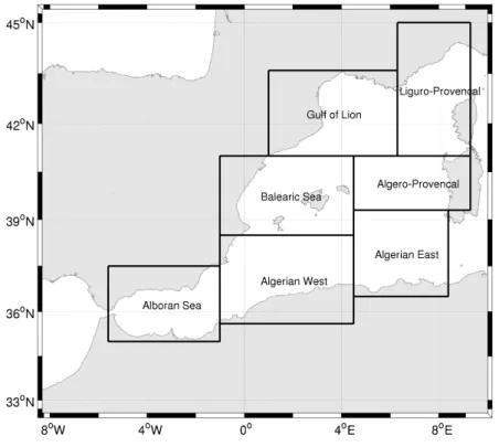
(28) 14. 2.3. GENERAL CIRCULATION AND WATER MASSES. Figure 2.2: Different areas of the WMed as defined by Manca et al. (2004). et al. (2010) argue that the circulation is more complex, with wind-driven cyclones in the northwest Tyrrhenian (Marullo et al., 1994) that are coupled with an anticyclonic gyre in the center of the basin. In the Northern part of the basin, the main current is the Northern current which flows westward along the French coast in the Ligurian Provençal Basin, the Gulf of Lion and then the Spanish coast in the Balearic Sea. It is stronger and closer to the coast in winter while weaker and broader in summer due to its meanders (Conan and Millot, 1995; Birol et al., 2010). The current then splits into two branches, one going back along the Balearic northern shore (Ruiz et al., 2009a; Mason and Pascual, 2013) and the other flowing southward through the Ibiza channel (Pinot et al., 2002). This description of the general surface circulation is in agreement with the synthetic Mean Dynamic Topography (MDT) derived by Rio et al. (2014) (figure 4.1) which was obtained by combining hydrological profiles, model outputs, altimeter observations and drifting buoy velocities. Global circulation models have been shown to be able to reproduce correctly this circulation as shown by Vidal-Vijande et al. (2012) but they lack the reso-.
(29) CHAPTER 2. THE WESTERN MEDITERRANEAN SEA. 15. lution to reproduce mesoscale features.. 2.3.2. Water masses. Apart from the AW at the surface, whose origin, characteristics and circulation we have already described, there are several more characteristic water masses in the WMed (Nielsen, 1912). The Mediterranean Sea has several sites of convection where, in winter, cold and dry winds evaporate already denser water and create vertical mixing more or less deep that generate dense waters. The north of the Levantine basin is one of them. There, a layer 300-500m deep of salty water called Levantine Intermediate Water (LIW) is formed in winter under the action of northerly winds (Robinson et al., 1991). In summer, the surface layer warms up but the LIW stays at depth (200-400m) and spreads to the whole Mediterranean marking a maximum of salinity at these depths. After passing the strait of Sicily and going northward along the Italian coast, some of the LIW goes through the Corsica strait between Corsica and France to follow the path of the Northern current at depth. Yet the majority of these waters flows southward along the eastern coast of Corsica and Sardinia and enter our area of study through the Sardinia strait where they bifurcate northward to join the rest of the LIW at the southern coast of France (Millot, 1999). The other main convection site is the Gulf of Lion where the Western Mediterranean Deep Water (WMDW) is formed (Marshall and Schott, 1999). The process is separated into the preconditioning phase where the cyclonic circulation in the Gulf of Lion intensify bringing interior waters that are less stratified to the surface (”doming”) and increasing the inflow of salty LIW waters. Surface waters are also getting denser due to loss of temperature and water due to atmospheric forcings (evaporation). Then, strong cold and dry winds events coming from the north induce loss of buoyancy that destabilizes the water column and create powerful vertical mixing which can reach the bottom of the basin. The WMDW created then spread at the bottom of the basin as observed by Send et al. (1996) forming the bottom layer of the water column in the WMed. When the conditions are not sufficient to trigger the deep convection, the cooling induces nonetheless a mixing of the surface layer with the highsalinity LIW which form the Western Intermediate Water (WIW), both.
(30) 16. 2.4. MESOSCALE DYNAMICS. cooler and fresher than the LIW and therefore placed above it (Send et al., 1999). This water mass, first described by Salat and Font (1987), is advected southward by mode water eddies in the Northern Current (Pinot et al., 2002). In a recent study, Juza et al. (2013) described the formation and spreading of the WIW using a high resolution model of the WMed. They showed that this water mass can propagate southward into the Alboran Sea where it is detected as a minimum of potential temperature.. 2.4. Mesoscale dynamics. In the Western Mediterranean Sea, mesoscale activity is present albeit rather inhomogeneous as shown by the levels of EKE in altimetry data (Pujol and Larnicol, 2005) but also drifter data (Poulain et al., 2012). As explained in the Introduction (chapter 1), the Rossby radius is relatively small in this region which makes studying the mesoscale difficult and hence reveals the need for high resolution datasets. This explains why the most of the mesoscale dynamics of the basin have started to be described only recently. Small mesoscale features are difficult to observe but large ones such as the Alboran gyres or the Algerian eddies have been thoroughly studied through, firstly, ship-based hydrographic cruises and, later with the help of satellite sensing or autonomous vehicles (gliders). The development of higher resolution or better spatial and temporal coverage datesets have allowed to steadily improve our knowledge of the mesoscale in the WMed. However, still most of the knowledge we have of the mesoscale in the region comes from localized surveys or simulations that describe specific eddies or low resolution models that can only resolve the larger eddies.. 2.4.1. Alboran Sea. As presented in section 2.3, the Atlantic inflow that goes through the Strait of Gibraltar forms two large anti-cyclonic gyres at the entrance of the Mediterranean Sea (Vazquez-Cuervo et al., 1996; Viúdez et al., 1996; Allen et al., 2001). Even though these structures were known about for a relatively long time, the more recent satellite data have helped to better understand the dynamics of these mesoscale gyres. Using extensive in-situ profiles as well as Sea Surface Temperature (SST).
(31) CHAPTER 2. THE WESTERN MEDITERRANEAN SEA. 17. from satellites, Viúdez et al. (1996) made the first accurate description of the gyres. Then, with more in-situ data (moorings, current meters, tide gauges) and more satellite-based SST, Vargas-Yáñez et al. (2002) described two different regimes for the circulation in the basin, one with only the WAG in winter-spring and one with the two gyres in summer-autumn. This study was completed by Renault et al. (2012) who studied the annual and interannual variability of the gyres from altimetry maps. Ship measurements allowed Allen et al. (2001) to characterize the hydrography and vertical velocities in these gyres. Using a combination of in-situ data, SST from satellites and satellite altimetry, Flexas et al. (2006) discovered a migration of the WAG and discussed some hypotheses for its migration. In July 2008, an experiment described by Ruiz et al. (2009b) involving new glider technology that helped to calibrate altimetry data in the eastern Alboran Sea was used to evaluate vertical velocities in the gyres. Combining the high resolution hydrographic data from the glider and satellite altimetry they were able to estimate the vertical exchanges to be about 1 m per day in the gyres. Recently, Peliz et al. (2012) made a realistic high resolution (2 km) simulation of the basin and used it to study the mesoscale dynamics (Peliz et al., 2013). They confirmed the two modes described by Renault et al. (2012) and examined the WAG migration and its impact on the transition between the two regimes. A study on the mesoscale eddies in this region was also conducted where they found that the generated eddies were small (mean radius of 13 km), short lived (less than 3 weeks), more likely to be cyclones and they were generated preferably when the two gyres were not present. The eddies were found to be generated mostly by instabilities of the jet and strong currents along the shore and at the Strait of Gibraltar.. 2.4.2. Algerian Basin. The Algerian basin is located at the south of the WMed along the Algerian coast and can be separated into a western and an eastern part (see figure 2.2). In this region, the Algerian current is highly unstable and the circulation is dominated by strong and large mesoscale eddies (Olita et al., 2011). Such mesoscale eddies, known as Algerian Eddies have been observed since the 1970s (Katz, 1972; Burkov et al., 1979) and have been described from in-situ data from oceanographic cruises (Benzohra and Millot, 1995).
(32) 18. 2.4. MESOSCALE DYNAMICS. or drifting buoys (Font et al., 1998). The launch of earth observing satellites enabled an easier observation of these structures as well as the possibility to follow them using satellite infrared images (Millot, 1985) or altimetry (Ayoub et al., 1998). The combination of these datasets with other sensors like drifting buoys (Salas et al., 2002; Font et al., 2004) showed the reliability of the satellite sensors and their potential to describe these large mesoscale eddies. Their influence on biology has also been studied using cruise data (Morán et al., 2001). With an extent that can reach 1000 m as observed by Ruiz et al. (2002), these features have diameters of about 100-200 km and their lifetime ranges from several months up to 3 years (Puillat et al., 2002). Algerian eddies usually follow the main eastward flow, from which they obtain energy, until they detach from the coast and drift northward where they eventually arrive in the center of the basin. There, they tend to go westward and may go back into the Algerian current and thus make a loop (Puillat et al., 2002). When the eddies detach from the Algerian coast, they transport water mass properties northward instead of eastward by the current. Isern-Fontanet et al. (2004) used altimetry in combination with hydrographic data from cruises to describe the spatial 3D structure of these large anticyclonic eddies. The Algerian mesoscale eddies are usually generated as a result of baroclinic instability (Millot, 1985; Beckers and Nihoul, 1992).. 2.4.3. Algero-Provençal basin. In the Algero-Provençal basin, there are no well defined mean currents. However, maps of altimetry derived EKE (see figure 4.15) show that transient features are common. In this part of the WMed, mesoscale activity is mainly associated with the large Algerian eddies that formed from the instabilities of the Algerian current that goes northward into this basin. There are also anticyclones called Sardinian eddies that are at an intermediate depth, formed by intermediate water coming westward from the Sardinian Strait and going northward along the Sardinian coast. These are generated at 39◦ N and travel westward; their signature is difficult to differentiate from Algerian eddies without in-situ measurement of the characteristics of the eddy cores (Testor et al., 2005)..
(33) CHAPTER 2. THE WESTERN MEDITERRANEAN SEA. 2.4.4. 19. Liguro-Provençal basin and Gulf of Lion. The main permanent characteristic of the Liguro-Provençal basin and Gulf of Lion is the Northern current. Mesoscale activity has been observed in this region (Robinson et al., 2001) with a strong increase in autumn (Font et al., 1995). The Northern Current has been shown to make intrusions on the shelf which are responsible for exchanges between open waters and the shelf (Petrenko et al., 2005). Millot et al. (1980), with meteorological data from a station and satellite infrared images, determined the role of south-easterly winds in these intrusions. Analysing an improved coastal along-track altimetry product in the gulf, Bouffard et al. (2011) was able to observe these features in altimetry data which allows a better monitoring of them. On the western part of the current, anticyclonic mesoscale eddies have been detected by hydrological and current meter observations (Estournel et al., 2003; Millot, 1982). A project called LATEX, combining data from an inert tracer release (SF6), Lagrangian drifters, satellites and Eulerian moorings with numerical modelling, was initiated in 2008 to study these mesoscale dynamics. Results from the model (Hu et al., 2009), as well as the other sensors (Hu et al., 2011) give an improved picture of the mesoscale activity in this area. An anticyclonic eddy lasting at least 50 days was observed with a radius of about 20 km, similar to what had been also observed in 2001. With the help of the high resolution (3 km to 1 km) model, the death of the eddy was linked to its interaction with the Northern Current while its formation was hypothesized to be due to the combined effect of strong Tramontane winds and the Northern Current (Millot, 1982; Hu et al., 2009). Rubio et al. (2009) used a high resolution regional model of the Northwestern Mediterranean Sea to study the generation and evolution of eddies in this basin. They found two different sites of eddy formation : near the city of Marseilles and at the same place as the LATEX experiments (Roussillon site). In the Marseilles site, the generation of eddies is related to the current that separates from the coast and creates eddies from barotropic instabilities. In the Roussillon site, the separation of the current is also the origin of the eddies but the wind also plays a role and the generation of the eddies is a combination of barotropic and baroclinic instabilities. (Garreau et al., 2011) using another high resolution model explained the.
(34) 20. 2.4. MESOSCALE DYNAMICS. generation of the LATEX eddies and also how they are linked to offshore eddies propagating in the Catalan seas.. 2.4.5. Balearic Sea. In the Balearic Sea, the general circulation (Font et al., 1988) is composed of the Northern Current flowing along the Catalan coast that then separates in two branches, one going through the Ibiza channel (Pinot et al., 2002) and the other recirculating into the Balearic Current, which flows eastward along the Northern shore of the Balearic Islands (Mason and Pascual, 2013). This circulation is modulated by mesoscale activity that, at first, was underestimated (La Violette et al., 1990) but later was found to be similar to the Algerian current (Garcı́a et al., 1994). In the Balearic Current, many studies have shown the existence of mesoscale structures by analysing satellite data, drifting buoys, oceanographic cruises or gliders (e.g. Pinot et al. 1995; Ruiz et al. 2009a; Bouffard et al. 2010). In particular, Pascual et al. (2002) used SST data from satellites as well as SLA from altimetry to infer the formation, life and decay of a strong anticyclone north of Mallorca that blocked the usual circulation in the Balearic Sea. A smaller anticyclonic eddy was also found in this area by Pascual et al. (2010) in 2009 during a multi-sensor experiment. More recently, Amores et al. (2013) used a mooring to describe the characteristics of an eddy appearing in the same area. The eddy evolved from a front detected and described by Balbı́n et al. (2012) using Conductivity Temperature Depth (CTD), satellite and mooring data. The size of these eddies ranged between 15 km (Pascual et al., 2010; Amores et al., 2013) and 100 km (Pascual et al., 2010). The formation of such eddies has been hypothesized to be due to instabilities of the Balearic Current, the formation of a meander and then a coherent vortex (Amores et al., 2013) for the smaller eddies. Direct action of the wind can also transmit anticyclonic vorticity from the negative curl associated with the shear of the Mistral downstream of the Pyrenees forming the larger eddy as proposed by Pascual et al. (2002) and Mason and Pascual (2013)..
(35) CHAPTER 2. THE WESTERN MEDITERRANEAN SEA. 2.5. 21. Recent advances in modelling and global observations of the mesoscale in the WMED. 2.5.1. Observing systems. As stated earlier, the Mediterranean Sea is an area that has been intensively investigated due to its unique location and importance for a large population. The mesoscale dynamics can be and have been investigated by very diverse observing systems. 2.5.1.1. Ships surveys. First, there are the regular ship cruise campaigns that can be designed to observe the mesoscale by doing high density CTD sampling in small areas allowing the construction of a 3D image of the ocean state. As an example, in a campaign in May 2009, Pascual et al. (2010) were able to study an eddy event occurring at the north shore of Mallorca. The dynamic height computed from the ship CTDs allows a reconstruction of this eddy which was also detected in SST from satellite, drifter data and gliders. Another example is the LATEX campaign mentioned earlier in which the combination of ship measurements consisting of Acoustic Doppler Current Profiler (ADCP) and CTD sensors as well as SST satellite images and Lagrangian drifter trajectories detected the presence of an eddy and enabled the study of its characteristics described in Hu et al. (2011). However, these cruises are costly and can only sample a small area of the ocean over a given time, as a larger area means lower sampling density or high inhomogeneity in time. Such cruises are useful to study a particular mesocale eddy or structure. 2.5.1.2. Surface drifters. Lagrangian floats are an inexpensive and convenient tool to study surface currents. They are buoys with a drogue at about 15 m depth that passively follow the horizontal flow at the surface. Their position is known via satellite and they can carry temperature or air pressure sensors. They can be deployed easily in high numbers and can provide information for large spatial domains. Poulain et al. (2012) compiled and analyzed a database of these drifters in the Mediterranean to study the mean circulation and energy. Despite these advantages, due to their nature, drifters cannot be.
(36) 22. 2.5. RECENT ADVANCES IN MODELLING AND GLOBAL OBSERVATIONS OF THE MESOSCALE IN THE WMED. controlled and the sampling is highly inhomogeneous. These drawbacks preclude a global analysis of the mesoscale from drifter data.. 2.5.1.3. Moorings. Moorings with temperature, salinity or current sensors produce a very high temporal resolution view of the water column. These time-series have the temporal resolution (less than an hour) to detect mesoscale and submesoscale dynamics and have successfully been used to describe mesoscale eddies such as the work by Amores et al. (2013) or Zhang et al. (2013). Amores et al. (2013) studied data from a mooring north of Mallorca revealing the passage of an eddy that affected the whole water column for one month. The analysis of the data showed that the eddy’s core was formed by WIW. However, the observational data provided by this sensor is limited to a single point in space and therefore can only describe temporal and, to a more limited degree vertical variability. It has to be combined with other observing systems as it is too limited for a regional monitoring of the mesoscale.. 2.5.1.4. Gliders. Underwater gliders are autonomous vehicles with various sensors (CTD, oxygen sensor, chlorophyll,...) that can sample 2D fields with high spatial resolution (1 km) down to depths typically around 1000 meters along a previously defined saw-tooth trajectory. They can be deployed to efficiently sample the mesoscale activity within a predefined area as shown by L’Hévéder et al. (2013) in an Observing System Simulation Experiment (OSSE). However, gliders are expensive and only cover relatively small areas for a limited time. The data from a glider in combination with along-track altimetry enabled Bouffard et al. (2010) to describe an intense mesoscale eddy found in the Balearic Sea. Heslop et al. (2012) used a repetitive sampling of the Ibiza Channel to characterize the transport and the mesoscale activity in the strait. The dataset provided very useful information but the temporal resolution was still not sufficient to fully characterize the mesoscale..
(37) CHAPTER 2. THE WESTERN MEDITERRANEAN SEA 2.5.1.5. 23. Coastal radars. High frequency (HF) radars measure wave heights but also surface currents by measuring the Doppler shift of the Bragg scattering of the radar signal. Positioned in coastal areas they are adequate to monitor mesoscale activity providing a high spatial (3 km) and temporal (20 minutes) resolution view of the currents (Quentin et al., 2013). However, HF radar ranges are limited (50-100 km) and thus they are only viable for coastal studies. 2.5.1.6. Observatory centers. As all these observing systems have different strengths and weaknesses, high quality information can be extracted from the combination of multiple sensors (Pascual et al., 2010; Ruiz et al., 2009a). However, such studies tend to be local and cover short periods of time. Two main observatory centers, located in the Western Mediterranean are dedicated to the continuous monitoring of the basin: MOOSE (Mediterranean Ocean Observing System for the Environment) for the Northern part of the basin and SOCIB (Sistema d’observació i predicció costaner de les Illes Balears) for the Balearic Sea. These observatory centers aim to develop a network of observations combining all the observations cited above and their objective is to make the data easily available for the user. The MOOSE network comprises two HF radars located at the south of France, gliders which sample regularly two transects in the Gulf of Lion, at least two deep moorings in the region, coastal stations of meteorology and regular ship campaigns. The SOCIB facility has a HF radar on the Ibiza and Formentera islands, several gliders which regularly sample the Ibiza Channel and also perform one-time missions (Troupin et al., 2014), drifters that are launched for campaigns, an oceanographic ship and an operational forecast model of the Western Mediterranean Sea at 1/32◦ . Efforts made with these initiatives greatly improve our knowledge of the Mediterranean Sea and its dynamic at various scales including mesoscale. Still, these observation systems are not suited for our goal of a systematic characterization of the region which need a relatively homogeneous spatial and temporal coverage at high resolution. 2.5.1.7. Satellite observations. In order to make synoptic observations of mesoscale activity in the Western Mediterranean, remote sensing data from satellites is a promising alterna-.
(38) 24. 2.5. RECENT ADVANCES IN MODELLING AND GLOBAL OBSERVATIONS OF THE MESOSCALE IN THE WMED. tive as it provides very good spatial coverage and temporal frequency. Two broad type of sensors are placed on these satellites, radiometers (passive sensor) and radars (active sensor). They have to work at wavelengths that are not absorbed by the atmosphere and therefore the spectral bands available are visible/near infrared (ocean color), thermal infrared (SST) and microwaves (microwave radiometry for SST, radars for Sea Surface Height (SSH)). Images from visible/near infrared and thermal infrared have high spatial resolution and have been used in many studies, many of them which we already described in the previous section. Yet, these datasets have two main limitations. First, the observed quantity is only a tracer and for SST, not a passive one which means that the motions can not be directly recovered. Methods have been constructed such as the one proposed by Vigan et al. (2000) to compute velocities from SST data but they are not completely reliable. Gaultier et al. (2013) proposed an innovative approach combining these images with radar altimetry from satellite to generate high resolution altimetry data. Yet this method is also limited for our objectives by the second limitation of these datasets, which is the fact that they are sensitive to cloud coverage. When there are clouds in the area, the ocean color or SST information cannot be retrieved, preventing the consistent analysis we want to perform. Microwave radiometry are not affected by clouds and thus provide an homogeneous coverage of the ocean but it has a much coarser resolution of about 50 km (Wentz et al., 2000) which is not sufficient to study mesoscale in our region. The last available remote sensing dataset is then radar sea surface height from altimetry that we used in our study and will describe below.. 2.5.2. Altimetry. 2.5.2.1. Along-track data. Radar altimeter from a satellite allows to observe the dynamic topography of the ocean or SSH by calculating the propagation time of a transmitted signal and then the distance R between the satellite and the sea. The dynamic height is deduced by knowing the satellite distance to an ellipsoid reference (S) and the geoid distance to this ellipsoid (hg ): : η = S − h − hg. (2.1).
(39) CHAPTER 2. THE WESTERN MEDITERRANEAN SEA. 25. The value of S is determined by the combination of several locating systems like the Global Positioning System (GPS) or the Doris system, a network of 50 ground beacons, worldwide, transmitting to the satellite which use Doppler shift to accurately know its velocity and then its position by dynamic orbitography models. The Earth’s geoid is the SSH without any disturbance (current, tide, wind,...) only due to difference of gravity. Estimating this geoid has been the goal of two satellite missions, first GRACE (Gravity Recovery and Climate Experiment) launched in 2002 and GOCE (Gravity field and steadystate Ocean Circulation Explorer) launched in 2009. GRACE data has a horizontal resolution of around 500 km (Tapley et al., 2003) for the geoid which is not enough for our purpose. GOCE has a higher horizontal accuracy of 100 km but is still not sufficient for mesoscale in the WMed. The solution to this limitation has been to substract the temporal mean of the observed SSH to obtain the Sea Level Anomaly (SLA) which is the time evolving part of the SSH. The SSH is then reconstructed by adding the MDT, the mean value of the SSH, to the SLA in order to obtain the total height of the sea surface. A description of how the MDT is computed for the Mediterranean is presented in section 4.2. Several corrections need to applied to the raw signal in order to use it for geophysical applications. The first corrections are applied in order to correct the errors due to the signal atmospheric propagation. - Ionosphere : When the signal passes through the ionosphere (70 km to 1000 km), its speed is reduced due to dispersion which imply an error in the distance δR = Af with A a value characteristic of the state of the ionosphere and f the frequency of the signal. Since δR depends on the frequency, the solution is to send 2 signals with different frequency and the difference in the measured distance allows to find the value of A. The positioning system (Doris) can be used in complement as it measures the correction between the satellite and a station on Earth. - Wet troposphere : The troposphere contains large quantities of water which induce a delay of the signal. Since the medium is not dispersive, the corresponding error of distance does not depend on the frequency and we cannot use the same method as for the ionosphere. The water vapor corrections are made based on multi-frequency mi-.
(40) 2.5. RECENT ADVANCES IN MODELLING AND GLOBAL OBSERVATIONS OF THE MESOSCALE IN THE WMED. 26. crowave radiometers. - Dry troposphere : Other gases such as nitrogen or oxygen can modify the propagation of the signal in the troposphere. For these corrections, a meteorological model of the area is used to estimate the correction. Then, corrections directly linked to the geophysical application of the user are applied. - Sea state bias : When the signal arrives to the sea surface, it is reflected both by wave troughs and wave crests but dispersion at wave crests is stronger due to the convexity of the surface (Fu et al., 1994). The signal has therefore a bias towards troughs and is corrected with an estimation of the sea swell by the dispersion of the return signal (Gaspar et al., 1994). - Tides : The tide signal is removed from the raw signal with a tide model. - Inverse barometer : Variations of atmospheric pressure over the ocean create a variation of the SSH. Since these variations are not related to the oceanic circulation, this effect is removed for low frequencies by an inverse barometer correction based on surface pressure fields from atmospheric models. For the high frequencies variations, the MOG2D barotropic correction (Carrère and Lyard, 2003) is used which takes into account wind and pressure effects from the European Centre for Medium-Range Weather Forecasts (ECMWF) analysis. MOG2D correction has been shown to improve representation of high frequency effects on sea level (Pascual et al., 2008). Finally correction of the orbit errors have to be accounted for. A global multi-mission crossover minimization is performed as proposed by Le Traon and Ogor (1998) on the data. 2.5.2.2. Gridded fields. The raw information given by the satellite is the SLA along its track which is then optimally interpolated to produce the 2D maps containing the signature of mesoscale eddies (Le Traon et al., 1998) (see section 4.2 for a description of the dataset in the Mediterranean)..
(41) CHAPTER 2. THE WESTERN MEDITERRANEAN SEA. 27. On figure 2.3, the satellite missions that can be used in the interpolation are summarized. These altimeters are on 3 different types of orbits with different repeat period and distance between neighboring tracks. The Geosat missions have a repeat period of 17 days and a distance between tracks of 1.45◦ or 125 km at the Mediterranean latitude, then ERS/ENVISAT satellites have a longer period of 35 days and a small distance inter-track of 0.7◦ or 60 km, finally TOPEX/Poseidon and Jason altimeters have a short period of 10 days but a high inter-track distance of 2.8◦ or 240 km. As indicated in figure 2.3, the number of satellites available for the Optimal Interpolation (OI) is not the same throughout the 1992-2012 period with, for example, high density (four satellites) between 2002 and 2005 and lower density (two satellites) between 1992 and 2000. The density of tracks in the Mediterranean for the two configurations is shown in figure 2.4. In the worst case (two satellites), we see that the distance between two tracks is irregular and can be quite large (reaching 100 km) but in the best case (four satellites), the distance between the track is much smaller and the distance between one point and the nearest track does not exceed 50 km. In figure 2.5, we present the evolution of this distance over the WMed, it shows that even though the satellite constellation changes, the distance stays below 50 km for 90% of the domain.. Figure 2.3: Overview of the satellite altimeters missions.. To compute the gridded maps, the OI uses correlation scales adapted to this distribution of tracks as described in Pujol and Larnicol (2005) (100.
(42) 28. 2.5. RECENT ADVANCES IN MODELLING AND GLOBAL OBSERVATIONS OF THE MESOSCALE IN THE WMED. Figure 2.4: Distance between grid point and next available tracks in the optimal interpolation for 2 different configurations. The maps are plotted for the same particular day as in figure 1 of Pascual et al. (2007) (12 November 2002). The distance is shown in kilometers.. km for spatial correlation and 10 days for temporal). The spatial correlation function is the one proposed by Arhan and De Verdiere (1985) which correspond to a smoothing of around 50 km (see Annex C). These correlation scales, and more fundamentally the distance between the tracks, are strong limitations in terms of spatial resolution of the altimetry maps. The observable scales in altimetry are therefore limited and only large (>30km) and relatively stable mesoscale structures can be acurately detected. This is particularly crucial for the study of mesoscale in the WMed since the structures observed have smaller dimensions than in the global ocean. Other limitations can include errors of measurement, atmospheric corrections or orbital errors..
(43) CHAPTER 2. THE WESTERN MEDITERRANEAN SEA. 29. Figure 2.5: Evolution of the mean distance between gridpoints and the next available track in the WMed. The distance is in kilometers.. 2.5.2.3. Studies. Concerning remotely sensed global observations of eddies in the Mediterranean, the work of Iudicone et al. (1998) opened the field. Using the first altimeter data from TOPEX/POSEIDON, they described the mesoscale features of the Mediterranean finding high seasonal variability, and northward transport of momentum due to the Algerian eddies. Later, a study by Isern-Fontanet et al. (2006) made the first automated detection of eddies in the Mediterranean that he applied to 7 years of gridded altimetry data. They used the Okubo-Weiss method that relies on the eponymous parameter which gives information on the relative dominance of strain and vorticity in the fluid. The detected vortices have a mean size of 30 km with a standard deviation of 25 km, the bigger eddies corresponding to stronger ones. Selecting only the strongest eddies (amplitude above twice the standard deviation of the Okubo-Weiss parameter), they did not find any seasonal variability. Finally, the path of the detected eddies is examined showing some clear patterns of propagation.. 2.5.3. Modelling. Concerning numerical modelling, efforts have increased a lot in recent years. Two different type of numerical models have been designed..
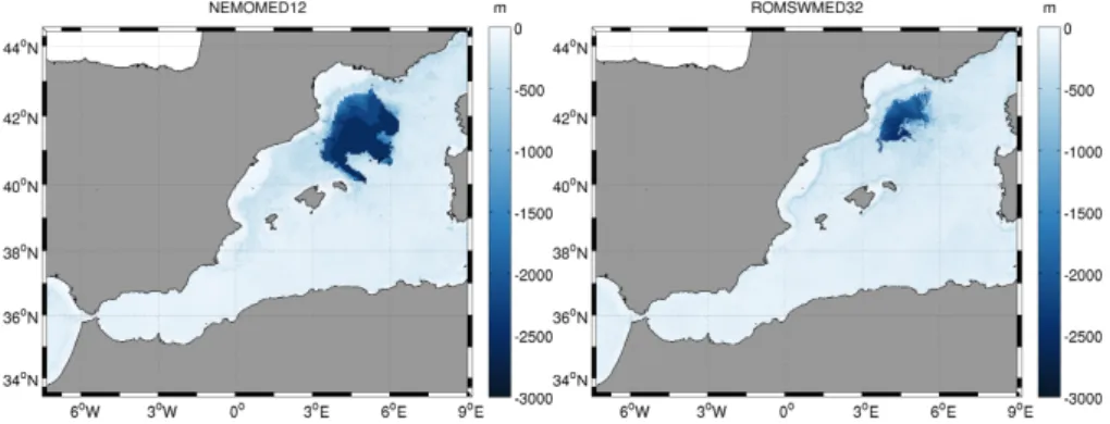
(44) 2.5. RECENT ADVANCES IN MODELLING AND GLOBAL OBSERVATIONS OF THE MESOSCALE IN THE WMED. 30 2.5.3.1. Long-term simulations. First, long term simulations of the Mediterranean Sea exist aiming at interannual and climatic studies. In this category, there is NEMOMED12 developed by Beuvier et al. (2012) with the Nucleus for European Modelling of the Ocean (NEMO, Madec and the NEMO Team 2008) model. This model is applied to the Mediterranean with a 1/12◦ horizontal resolution (with a NEMOMED36 in preparation at 1/36◦ horizontal resolution) and ran for a period of 50 years in hindcast (without assimilation). This simulation covers the period desired for our study but the resolution (about 8 km) is not sufficient to fully resolve the mesoscale in the region. Then there is the reanalysis simulations that include data assimilation. The operational models MFS (Mediterranean Forecasting System) has a resolution of 1/16◦ and provides a reanalysis of the last 25 years with data assimilation. MERCATOR also offers a reanalysis of the last 20 years of the global ocean (including the Mediterranean Sea) at a resolution of 1/12◦ . These simulations are still too coarse and furthermore does not serve our purpose since the use of data assimilation prevents a study of the processes involved in the mesoscale dynamics as it does not let the model run freely. 2.5.3.2. Short studies. On the other hand, high resolution models are designed for smaller areas and shorter time spans. One example is the SYMPHONIE model that runs for the Gulf of Lion area at a resolution of 1 km (Marsaleix et al., 2006). Herrmann et al. (2008) studied the impact of the atmospheric resolution for the deep convection in the Gulf of Lion with this model. Another high resolution simulation is GLAZUR 64, based on the NEMO code that covers the North Western Mediterranean with an horizontal resolution of 1/64◦ and 130 vertical levels. The simulation was run for several years and has been used, in combination with in-situ data, to study an anti-cyclonic eddy in the Gulf of Lion (Guihou et al., 2013). The regional model MARS3D developed by Lazure and Dumas (2008) has been also applied at a horizontal resolution of 1.2 km in the Northern WMed in a study we discussed above by Garreau et al. (2011). In the Alboran Sea, the simulation cited earlier by Peliz et al. (2013) using the ROMS core revealed insights into the mesoscale activity in the Alboran Sea. The lack of an existing simulation with a high enough resolution to de-.
(45) CHAPTER 2. THE WESTERN MEDITERRANEAN SEA. 31. scribe the mesoscale dynamics over the entire WMed motivated us to design our own simulation. The simulation covers the Western Mediterranean and is run for a long period of time in order to have statistically robust results and to study annual and inter-annual variability. The details of this model are summarized in chapter 3..
(46) 32. 2.5. RECENT ADVANCES IN MODELLING AND GLOBAL OBSERVATIONS OF THE MESOSCALE IN THE WMED.
(47) Chapter 3 A high resolution model of the area Contents 3.1. Objective . . . . . . . . . . . . . . . . . . . . . . .. 34. 3.2. ROMS model . . . . . . . . . . . . . . . . . . . . .. 35. 3.3. 3.2.1. Primitive equations . . . . . . . . . . . . . . . . .. 35. 3.2.2. Vertical boundary conditions . . . . . . . . . . .. 36. 3.2.3. Terrain-following coordinate system . . . . . . .. 37. Physical parameterizations . . . . . . . . . . . . .. 40. 3.3.1. Advection schemes . . . . . . . . . . . . . . . . .. 40. 3.3.2. Boundary layer parameterization . . . . . . . . .. 40. 3.4. Spatial and temporal discretization . . . . . . . .. 41. 3.5. Topography . . . . . . . . . . . . . . . . . . . . . .. 42. 3.6. 3.7. 3.5.1. Pressure gradient error . . . . . . . . . . . . . . .. 42. 3.5.2. Gibraltar . . . . . . . . . . . . . . . . . . . . . .. 45. Initial state and boundary conditions . . . . . .. 47. 3.6.1. NEMOMED12 simulation . . . . . . . . . . . . .. 47. 3.6.2. Initial conditions . . . . . . . . . . . . . . . . . .. 48. 3.6.3. Boundary parameterization . . . . . . . . . . . .. 48. Atmospheric forcings . . . . . . . . . . . . . . . .. 49. 3.7.1. Flux forcing . . . . . . . . . . . . . . . . . . . . .. 49. 3.7.2. Bulk parameterization . . . . . . . . . . . . . . .. 50. 33.
(48) 34 3.8. Rivers . . . . . . . . . . . . . . . . . . . . . . . . .. 50. 3.9. Set of simulations . . . . . . . . . . . . . . . . . .. 51. 3.10 Computing resources . . . . . . . . . . . . . . . .. 51. 3.11 Conclusion. 54. . . . . . . . . . . . . . . . . . . . . . ..
Figure
+7
Documento similar
MD simulations in this and previous work has allowed us to propose a relation between the nature of the interactions at the interface and the observed properties of nanofluids:
A catchment model for river basins and a hydrodynamic model were combined in order to simulate the spreading of the turbidity plume produced by sediment discharges from the
The expansionary monetary policy measures have had a negative impact on net interest margins both via the reduction in interest rates and –less powerfully- the flattening of the
- Competition for water and land for non-food supply - Very high energy input agriculture is not replicable - High rates of losses and waste of food. - Environmental implications
Keywords: Metal mining conflicts, political ecology, politics of scale, environmental justice movement, social multi-criteria evaluation, consultations, Latin
Recent observations of the bulge display a gradient of the mean metallicity and of [Ƚ/Fe] with distance from galactic plane.. Bulge regions away from the plane are less
(hundreds of kHz). Resolution problems are directly related to the resulting accuracy of the computation, as it was seen in [18], so 32-bit floating point may not be appropriate
Even though the 1920s offered new employment opportunities in industries previously closed to women, often the women who took these jobs found themselves exploited.. No matter
