Should cohesion policy focus on fostering R&D?
Evidence from Spain
Adolfo Maza*, José Villaverde*, María Hierro*
ABSTRACT: Over the last decades, there has been a vast amount of literature on the subject of Research and Development (R&D) expenditure as a main driver of economic growth, both at national and sub-national levels. This being so, the main purpose of this manuscript is to investigate the role played by R&D as a cohesion instrument. To accomplish this aim, the paper assesses the link between patents (as a proxy for R&D) and economic growth across the Spanish provinces (NUTS3) over the period 1995-2010. In other words, we want to evaluate whether provinces with high patent production grow at a higher rate than those with low innovative performance. In addition, we want to test for the presence of spatial spillovers, and to assess if the effect of patents on economic growth depends on the development degree of provinces. The results show, firstly, that patents act as a growth driver. Secondly, that there is no evidence of spatial spillovers. And, thirdly, that the effect of patents on growth seems to be higher for developed than for less developed provinces. In view of these findings, major efforts should be devoted to promote a cohesion policy focused on R&D investment in the less developed territories. JEL Classification: O30; O40; O11; R11.
Keywords: patents; economic growth; Spanish provinces.
¿Debería la política de cohesión centrarse en el fomento de la I+D?: Evidencia para España
RESUMEn: Durante las últimas décadas la literatura sobre los gastos en investi-gación y desarrollo (I+D) como motor de desarrollo, tanto a nivel nacional como regional, ha crecido de forma notable. En este contexto, el objetivo de este trabajo es examinar el papel jugado por los gastos en I+D como instrumento de cohesión. Para ello, el trabajo evalúa la conexión entre patentes (como proxy de gastos en I+D) y el crecimiento económico entre las provincias españolas (NUTS3) durante
Received: 14 march 2014 / Accepted: 30 june 2014.
We would like to thank two anonymous referees for their helpful comments and suggestions. The usual disclaimer applies.
* Department of Economics. University of Cantabria. Av. Los Castros, s/n. 39005 Santander (SPAIN). E-mail: [email protected]; [email protected]; [email protected].
el periodo 1995-2010. En otras palabras, queremos averiguar si las provincias con mayor número de patentes crecen a un ritmo más alto que aquéllas con poco impul-so innovador. Además, el trabajo analiza la presencia de efectos desbordamiento, así como si el efecto de las patentes sobre el crecimiento depende del grado de desarrollo de cada provincia. Los resultados ponen de relieve, primero, que las patentes impulsan el crecimiento. Segundo, que no hay evidencia que apoye la existencia de efectos desbordamiento. Tercero, que el efecto de las patentes sobre el crecimiento parece ser mayor en las regiones más desarrolladas que en la menos desarrolladas. De acuerdo con estos resultados, una política de cohesión enfocada en la inversión en I+D en las regiones menos desarrolladas parece ser necesaria. Clasificación JEL: O30; O40; O11; R11.
Palabras clave: patentes; crecimiento económico; provincias españolas.
1. Introduction
The existence of large and persistent regional disparities constitutes one of the main traits of the European Union (EU). As these disparities might pose some pro-blems to the process of European integration, their analysis and, correspondingly, the issue of how to deal with them has caught the attention of both academics and policy makers since at least the 1970’s, spawning a large theoretical and empirical research. In truth, this analysis revolves around a simple but critical question: why some terri-tories are rich and others are not? Put it other way, it discusses on the main sources of economic growth.
Among these sources, Research and Development (R&D) investment clearly stands out. There is a general consensus on the fact that disparities are mainly explai-ned by differences in productivity, and that these differences are, to a great extent, due to the development of new technologies as well as the capacity of regions to pro-fit from technology and, eventually, to harvest the benepro-fits of investments on R&D. That is to say, there is a well-defined strand of research confirming the relevance of technological progress as a growth engine and, consequently, of R&D as a key ele-ment in not only regional but also national and European-wide growth policies 1. The-refore, remarkable efforts have been displayed by different governments to increase the expenditure on R&D as a percentage of GDP, especially in the last decades.
Bearing these considerations in mind, the aim of this paper is to assess the perti-nence of the use of R&D investments not only as a growth driver but also as an ins-trument of the cohesion policy, let’s say a potential cohesion enhancer. But, how can we accomplish these two goals together? To do that, and although we are conscious of their limitations, we employ (both standard and spatially) conditioning beta-conver-gence approaches. By using these approaches we can establish whether, or not, regions that allocate a larger share of output to R&D grow at a higher rate than those with a
poor innovative performance and, by doing that, we also intend to estimate the poten-tial contribution of R&D investments to convergence or cohesion. Additionally, the paper addresses two closely related issues. Firstly, and taking into account a relatively new and important branch of the literature —the New Economic Geography (NEG) models inspired on the ground-breaking paper by Krugman (1991)—, it studies the interaction of R&D activities in one place with those in another 2. This is an extremely important topic (see e.g. Funke and Niebuhr, 2005), because this kind of intangible as-sets are specially pruned to the presence of spatial spillovers 3. Then, it also examines, by employing a spatially conditioning beta-convergence approach, whether the increa-se in R&D in a province positively affects the rate of economic growth of its neigh-bors. Secondly, and due to the fact that previous papers have shown that the effect of R&D expenditures on economic growth could depend on the development level of the areas where they are conducted, the paper also tests this hypothesis by using a set of interaction variables (combining R&D investments and the level of per capita GDP).
Regarding data, this paper takes the Spanish case as a sort of laboratory. To be precise, we use a sample of 50 Spanish provinces (excluding Ceuta and Melilla) over the period 1995-2010 and, due to R&D data unavailability at provincial level 4, we employ patent data (Patent Co-operation Treaty (PCT) patent applications per million inhabitants) as a proxy for R&D expenditure. Data about patents come from the Main Science and Technology Indicators databank provided by the OECD. Other data sources, such as Eurostat and IVIE, are also employed for the inclusion of some control variables in the study.
Bearing these considerations in mind, the rest of the paper is organized as follows. Section 2 presents a succinct review of the theoretical framework regarding the link between R&D and economic growth/convergence. Section 3 reviews the empirical literature devoted to the relationship between R&D and economic growth. Section 4 describes, in a concise way, the provincial distribution of patents in Spain. After that, Section 5 assesses the role played by patents as an engine for economic growth and convergence, the existence of spatial spillovers, and of differences according to the development level of provinces. Finally, Section 6 concludes and provides some les-sons and challenges for cohesion policy.
2 An extensive analysis of the inner connectivity of the Spanish Regional Innovation Systems has
been recently published by Alberdi Pons et al. (2014).
3 This is one of the reasons why the Lisbon Strategy focuses on R&D: EU countries/regions collect
well-being gains from each other’s investments on R&D.
4 It is worth noting that the analysis could be carried out at regional (NUTS2) level using R&D
investment data. However, we decided to run it at provincial (NUTS3) level because not only patents are commonly used as a proxy for R&D but mainly because we consider that an analysis at regional level suffers from serious problems of aggregation (the Spanish regions are of widely different sizes and encompass different number of provinces). Furthermore, the use of data at provincial level allows us to deal with to the potential existence of spatial dependence problems in the estimation of our model (as it is well-known that models including a spatial structure need a big sample), which could crucially affect the reliability of the results. Although at the same time we are aware that there are some papers indicating that the use of patents is not suitable because they are not a good proxy for R&D (e.g. Griliches, 1990; Sánchez
2. Theoretical literature review
Although the interest on R&D investments dates back to classical economists, in the modern era it was spurred by Solow’s (1956, 1957) work, that established the roots of the neoclassical growth theory. According to it, economic growth is explai-ned by factor accumulation and productivity growth, this last one being considered as an exogenous variable. The problem with this approach is that empirical literature has found, as mentioned in the Introduction, that the bulk of income differences among regions cannot be explained by differences in factor endowments, but by differences in productivity growth (Caselli, 2005). In other words, empirical evidence does not support the predictions made by Solow’s model.
Even though since Solow’s seminal papers several advances have been made, the next big step on the theory of economic growth did not take place until around mid-eighties with the endogenous growth theory (Romer, 1986, and Lucas, 1988). This theory tries to incorporate technological change, namely innovations, into eco-nomic growth models. Accordingly, productivity growth starts to be treated as an endogenous driver of growth. One of the reasons leading to this conclusion is that technological knowledge accumulated through the allocation of resources to R&D promotes productivity growth. As explained by Wei et al. (2001: 155), «the more resources allocated to R&D, the higher the incentive for firms to innovate, the grea-ter the firms’ abilities to create new technological ideas, and the higher the rate of growth a country will enjoy». Accordingly, differences in capabilities, resources and incentives to undertake innovative processes are expected to provoke large regional differences.
Following this line of research, during the last two decades there has been a surge in the literature devoted to assess the importance of investment in R&D as a source of economic growth. Among the most relevant papers, those by Romer (1990), with his product-variety model, Grossman and Helpman (1991), including spillover effects in the research sector, and Aghion and Howitt (1992), with their quality-ladder model involving creative destruction, stand out. As summarized by Barro and Sala-i-Martin (1995: 12), «in these models, technological advance results from purposive R&D activity, and this activity is rewarded by some form of ex-post monopoly power». These models conclude the existence of «scale effects» on innovation: the size of population affects long-run economic growth as any increase in population, ceteris paribus, raises the number of researchers.
Nevertheless, the prediction of «scale effects» in innovation based on the first generation of endogenous growth models was afterwards challenged, on empirical grounds, by Jones (1995), which developed a model that maintains the main featu-res of the R&D-based models but eliminates this «scale effect» prediction 5. In the
5 In this model economic growth is not endogenously determined but the result of population growth
same vein, many other models eliminating the «scale effect» have been proposed, among which those of Young (1998), Peretto (1998) and Howitt (1999) are probably the most prominent. These models, in short, include «horizontal» innovation as well as «vertical» innovation, so that the aggregate effect of any-one sector R&D inves-tments diminishes and, in consequence, the effect of population on resources devoted to R&D and economic growth vanishes (Garner, 2010).
In sum, from a theoretical perspective there are different approaches to assess the relationship between economic growth and R&D investments. Regarding neoclassi-cal models, and apart from the accumulation of factors, productivity gains induced by technological advances are a main source of economic growth. Therefore, the use of R&D investments as a way to boost productivity and, therefore, promote eco-nomic growth might even be considered an implicit finding from the neoclassical ap-proach. From the endogenous growth theory perspective, R&D is explicitly taken as a growth driver. Therefore, there seems to be a unanimous conclusion: there is a link between R&D expenditures and economic growth. With respect to this issue, Aghion and Howitt (2007: 93) indicate «that the contributions of capital accumulation and innovation to growth cannot be estimated without such a hybrid (neoclassical and
endogenous) theory».
3. Empirical literature review
Accordingly with the theory, the empirical evidence on the impact of R&D in-vestment on economic growth has generally found that this is positive and quite sig-nificant (see Nadiri, 1993, for a review). This notwithstanding, and as reported by Griliches (1992) in his analysis of R&D externalities, the range of elasticity estimates is very large, from a minimum of 20% to a maximum of 80%, depending on the firms, industries and countries under consideration 6. Drawing on this conclusion, Jones and Williams (1998) developed an endogenous-growth model to estimate the social rate of return of R&D 7 and, after calibrating it and showing that previous results repre-sented a lower bound, found that most decentralized economies undertake too little investment in R&D. In particular, they found that optimal R&D investment is about four times greater than actual spending 8.
With a more critical approach, other authors consider that the contribution of R&D to growth is somewhat uncertain as R&D investments cause not only positive externalities but also some negative spillovers. In this vein, Pessoa (2010) stresses the fact that relying on a «linear model» to capture the impact of R&D on economic growth is somewhat restrictive because of the many factors omitted in conventional
6 For a thorough review of the empirical literature on measuring the returns to R&D, see Hall et al.
(2009).
7 In this model the link between R&D and growth depends only on the production possibilities of
the economy.
8 By using a different approach —calibrating and endogenous growth model— Jones and Williams
regressions 9. More specifically, Pessoa (2010: 152-153) states that «if such factors have a clear effect on TFP and, at the same time, induce firms to invest in R&D, R&D intensity seems rather a proxy of the level of development than a cause of it». As a (partial) consequence of this, he shows, for a sample of 28 OECD coun-tries, that the average rate of GDP growth between 1995 and 2005 was not positively correlated to R&D intensity in the business sector, therefore casting some doubts about the conventional link between both variables. Similarly, papers by Dosi et al. (2006) and Braunerhjelm et al. (2010), for EU and OECD countries respectively, conclude that R&D efforts do not lead to sufficient economic growth. Ejermo et al. (2011), analyzing the R&D-growth paradox (R&D growth being higher than eco-nomic growth) for the Swedish case, observed that this is related to different sector growth patterns, with the fast-growing industries, not the traditional ones, being those that contribute the most to the paradox.
Another strand of empirical research, pioneered by Ulku (2004) in his work for 20 OECD and 10 non-OECD countries, challenges the assumption, employed when using OLS regressions, that the elasticity of output with respect to R&D is constant. According to some of these papers (see references in Wang et al., 2013) the rate of return of R&D crucially depends on the industries in which R&D takes place, with that corresponding to high-tech industries generating the highest returns, a result that is at odds with that of Ejermo et al. (2011). In accordance with this conclusion, Wang
et al. (2013) move a bit further and, by studying a sample of 23 OECD countries plus Taiwan, show that the impact of R&D investments in high-tech sectors is heteroge-neous across economies with different levels of per capita income. Similarly, a very recent research for the OECD countries (Westmore, 2013) casts some doubts about the robustness of the positive link between R&D and growth; more specifically, it states that the strength of the link depends on «well designed framework policies that allow spillovers to proliferate» (Westmore, 2013: 2), meaning that the impact may be heterogeneous across countries 10.
Apart from the type of industry or country that is undertaking the R&D inves-tment, its effect on the rate of economic growth might depend on the private or pu-blic character of the investment. Here the evidence is also mixed, and although the results are generally positive for both types of investment and as a total, there are some papers (Kealey, 1996) suggesting that public investment in R&D might de-ter growth. Sylwesde-ter (2001), in an analysis of the relationship between both public and private R&D investments and growth for a sample of 20 OECD countries, finds that albeit both coefficients are positive none of them are significant at conventional levels. When the relationship is estimated, however, just for the G-7 countries, the evidence of a positive effect is stronger, particularly regarding non-government R&D expenditures.
9 A recent paper by Strobel (2012) also stresses the different impact of R&D on growth by industry
type, that is, the non-linearity of the relationship between both variables.
10 Goel and Ram (1994) also concluded that, after controlling for several variables, there is a
posi-tive correlation (they do not talk about causality) between R&D investment and growth, but only for rich countries.
Within the bulk of papers adopting a country approach, it is important to mention a very recent and interesting one, by López-Rodríguez and Martínez (2014), which compares R&D and non-R&D innovation expenditures for a sample of 26 EU coun-tries. As these authors demonstrate, the effect of the former (R&D) is almost twice as larger as that of the latter (non-R&D). In addition, they show that the distance to the technological leader has a positive impact on growth.
From a regional perspective there are also many studies analyzing the effects of R&D on growth, particularly for the EU regions (see Sterlacchini, 2008, for some references). Among them, one of the most interesting from the point of view of this paper, as its econometric approach is roughly the same, is that by Sterlacchini (2008) for a sample of 197 NUTS2 regions over the period 1995-2002. By estimating a rather conventional beta-convergence equation in which, among others, patents are included as a control variable, two main conclusions arise. First, that R&D exerts a significant impact on GDP growth. And, second, that this effect is less significant for regions with relatively low levels of per capita income, which implicitly means that R&D works against convergence.
There are, however, much less studies about the R&D-growth link at regional level within a single country, and most of them are mainly interested in quantifying spatial spillovers. Among them, Funke and Niebuhr (2005) examine the (West) Ger-man case between 1976 and 1996 and, estimating a conventional beta-convergence model with spatial dependence, they achieve two relevant conclusions. First, that R&D has a positive impact on the rate of economic growth and, second, that inves-tment in R&D in a region positively affects income growth in other regions; this effect is, however, much stronger for geographically close regions than for the rest.
Finally, another interesting study, in between those of Sterlacchini (2008) and Funke and Niebuhr (2005) but with a somewhat different aim, is that by Bottazzi and Peri (2003). In this paper, and by means of using an innovation generating function for 86 EU regions for the period 1977-1995, the authors estimate the elasticity of innovation to R&D and find that it declines heavily with distance. From this conclusion, the impli-cation is obvious: as in Funke and Niebuhr (2005), spatial spillovers of R&D on growth only affect to the closest regions to those in which the R&D investment takes place.
4. The geographic distribution of patents across
the Spanish provinces
In their attempt to measure the innovative performance of economic areas, re-searchers have commonly followed one of these two strategies: First, the use of sta-tistics on R&D expenditures over GDP, considered as input indicators; second, the use of data on patent applications per million inhabitants as output indicators. As mentioned in the introduction, in this paper we have opted for using the number of patents per million of inhabitants for reasons of data availability. In any case, due to relatively high correlation usually found between both variables (see, for instance,
Bottazzi and Peri, 2003, and Bilbao-Osorio and Rodríguez-Pose, 2004) there is no reason to think that results are quite sensitive to the strategy adopted.
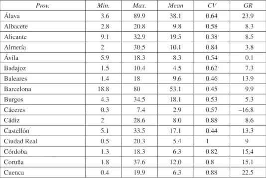
Table 1 displays some descriptive statistics based on the original data on patents for the Spanish provinces over the sample period. A first glance to this table reveals that important differences exist and, furthermore, that innovative performance increa-sed significantly over the sample period, the largest growth rates being recorded in Orense (28.5%) and Alava (23.9%). In fact, only four provinces registered a negative evolution: Cáceres, Las Palmas, Segovia and Teruel. But maybe the most important fact that emerges from this table is that the year-by-year data on patents are extre-mely volatile, with a coefficient of variation close to 0.5 for the whole country and even close to 1 for some Spanish provinces. As this fact makes difficult to model the evolution of patents, we decided to treat raw data by moving average techniques over the two neighboring points. As a result, from now on the new sample period ranges from 1996 to 2009 and these smoothed data are used in order to explore more deeply the main characteristics of the geographic distribution of patents across of Spanish provinces. Specifically, we focus our attention on three aspects of the distribution: inequality, external shape and spatial dependence 11.
Table 1. Patent applications per million inhabitants in the Spanish provinces (1995-2010)
Prov. Min. Max. Mean CV GR
Álava 3.6 89.9 38.1 0.64 23.9 Albacete 2.8 20.8 9.8 0.58 8.3 Alicante 9.1 32.9 19.5 0.38 8.5 Almería 2.0 30.5 10.1 0.84 3.8 Ávila 5.9 18.3 8.3 0.54 0.1 Badajoz 1.5 10.4 4.5 0.62 7.3 Baleares 1.4 18.0 9.6 0.46 13.9 Barcelona 18.8 80.0 53.1 0.45 9.9 Burgos 4.3 34.5 18.1 0.53 5.3 Cáceres 0.3 7.4 2.9 0.57 –16.8 Cádiz 2.0 28.6 8.0 0.88 8.6 Castellón 5.1 33.5 17.1 0.44 13.3 Ciudad Real 0.5 20.3 5.4 1.40 9.0 Córdoba 1.3 18.3 6.3 0.82 15.4 Coruña 1.8 37.6 12.0 0.80 15.1 Cuenca 0.4 19.9 6.3 0.88 22.5
11 We have also analyzed the polarization degree of the distribution. Although this information is not
Table 1. (Continue)
Prov. Min. Max. Mean CV GR
Girona 4.9 49.8 28.8 0.51 11.0 Granada 2.4 33.9 13.4 0.79 17.2 Guadalajara 1.5 23.7 11.6 0.59 2.9 Guipúzcoa 4.5 80.1 37.5 0.64 19.5 Huelva 1.1 23.2 7.5 0.71 12.5 Huesca 4.8 25.8 15.1 0.46 10.8 Jaén 0.3 13.5 4.1 1.13 15.5 León 3.3 16.3 8.8 0.44 7.0 Lleida 2.8 25.0 12.5 0.54 14.7 Rioja, La 0.9 34.8 15.3 0.69 10.4 Lugo 0.5 12.3 4.3 0.87 15.6 Madrid 13.2 67.3 36.3 0.50 11.1 Málaga 5.9 20.4 12.8 0.37 7.8 Murcia 0.3 23.0 11.9 0.59 12.4 Navarra 7.9 110.3 56.2 0.61 19.2 Orense 0.3 13.8 5.1 0.69 28.5 Asturias 2.5 23.3 10.1 0.66 12.5 Palencia 0.9 17.5 5.3 0.96 9.8 Palmas, Las 3.6 12.8 6.6 0.40 –1.4 Pontevedra 1.1 24.4 12.2 0.61 10.9 Salamanca 2.8 23.6 12.5 0.61 10.3 Tenerife 1.4 16.2 6.6 0.57 11.8 Cantabria 1.9 20.1 9.2 0.70 15.9 Segovia 1.6 19.4 7.6 0.58 –9.3 Sevilla 2.0 46.8 17.0 0.74 22.5 Soria 4.0 20.2 9.1 0.41 11.4 Tarragona 10.8 59.1 30.2 0.50 6.4 Teruel 1.4 23.7 10.1 0.58 –10.4 Toledo 0.8 27.0 12.9 0.62 9.0 Valencia 7.4 44.1 27.8 0.43 12.2 Valladolid 4.0 34.0 15.0 0.65 10.1 Vizcaya 5.6 54.7 23.3 0.66 14.2 Zamora 0.6 15.5 5.0 0.93 15.9 Zaragoza 7.1 77.7 33.2 0.73 16.1 SPAIn 7.1 38.4 22.8 0.48 11.9
Notes: GR = growth rate; CV = Coefficient of variation.
4.1. Inequality
First we study the evolution of provincial disparities in patent applications. Since there is no accepted best measure of inequality, we consider here the most commonly used inequality indicators: the coefficient of variation (CV), the Gini index (G), two versions of the Theil index (T(0) and T(1)) and a version of the Atkinson index (A(1)). All indices are independent of both scale and population size, and each one fulfills the Pigou-Dalton transfer principle (Cowell, 1995).
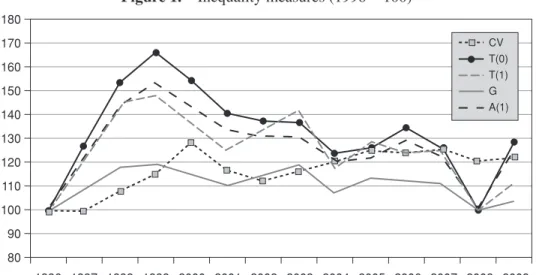
Results from applying the above mentioned inequality measures are shown in Figure 1. The main conclusion is that there was a high increase of inequality during the late 1990s, followed by a downward trend that has not been intense enough to reach in 2009 lower inequality levels than in 1996. Additionally, it can be observed that, even using moving averages, the time pattern of patents is rather volatile.
Figure 1. Inequality measures (1996 = 100)
CV T(0) T(1) G A(1) 180 170 160 150 140 130 120 110 100 90 80 1996 1997 1998 1999 2000 2001 2002 2003 2004 2005 2006 2007 2008 2009
Source: OECD and own elaboration.
4.2. External Shape of the Distribution
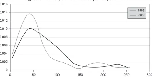
Supplementary information of the distribution can be inferred from the construc-tion of density funcconstruc-tions. This representaconstruc-tion, understood as a smoothed version of a histogram, provides a very simple yet highly intuitive graphical tool to visualize some general characteristics of any distribution, as well as to study the manner its external shape evolves over time. In order to estimate a density function we use a Gaussian kernel with optimal bandwidth according to the well-known Silverman’s rule-of-thumb (Silverman, 1986).
Figure 2 plots Spain’s patents distribution for the initial and final years of the sample period: 1996 and 2009. In this case, data are normalized by the Spanish average (Spain = 100). The figure shows that in 1996 the distribution is bimodal; by using Salgado-Ugarte et al. (1997) technique to identify the modes, it can be said that the main mode is located at 47.2% while the second is at 229.2% of the Spanish average. As for 2009, the distribution continues to be bimodal; now the differences are that the two modes have somewhat changed to the left (40.4 and 195.5% respec-tively) and that the mass of probability is more concentrated around the main one.
Figure 2. Density plots for relative patent applications
1996 2009 0.016 0.014 0.012 0.010 0.008 0.006 0.004 0.002 0 0 50 100 150 200 250 300
Source: OECD and own elaboration.
4.3. Spatial dependence
A first look at Spain’s map in both 1996 and 2009 (Figures 3a, 3b) reveals that, as ex-pected, innovative performance has tended to cluster in rich areas characterized by high economic dynamism, such as those in the North-East of the country. In addition, when Figures 3a and 3b are compared, it seems that spatial concentration has decayed at the end of the period; this conclusion stems from the fact that areas with similar values (high or low) of patent applications seem to be more spatially clustered in 1996 than in 2009.
As these conclusions are tentative at best, because they lack any sound statistical basis, to examine their real strength next we estimate the most widespread statistic in spatial analysis (ESDA): the Moran’s I statistic 12. Using the inverse of the
standard-12 This is expressed as follows (Anselin, 1988):
I t n w w y t t y t ij j i ij j i i j ( ) ( ) ( ) ( ) * * = − −
∑
∑
∑
∑
µ µ(( ) ( ) ( ) t y ti t i − ∑
µ 2where yi and yj are patent applications per million inhabitants of provinces i and j, respectively; m is the Spanish average; wij wij wij
j
*=
∑
are the standardized spatial weights describing the distance betweenprovinces i and j; and n is the number of provinces. In order to facilitate the interpretation of the statistic, the standardized value (z-value) is obtained. Accordingly, a significant positive (negative) value for the Moran’s I statistic will imply positive (negative) spatial association, herein interpreted to imply similar (dissimilar) values of patent applications per million inhabitants being clustered together in space.
Figure 3. Relative patent applications across the Spanish provinces (Spanish average = 100) 0-40 40-80 80-120 120-160 > 160 0-40 40-80 80-120 120-160 > 160
(a) Year 1996 (b) Year 2009
Source: OECD and own elaboration.
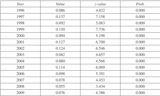
Table 2. Moran’s I statistic
Year Value z-value Prob.
1996 0.086 4.832 0.000 1997 0.137 7.158 0.000 1998 0.092 5.083 0.000 1999 0.150 7.736 0.000 2000 0.094 5.198 0.000 2001 0.127 6.700 0.000 2002 0.124 6.546 0.000 2003 0.082 4.657 0.000 2004 0.080 4.566 0.000 2005 0.114 6.089 0.000 2006 0.098 5.391 0.000 2007 0.078 4.453 0.000 2008 0.055 3.434 0.000 2009 0.076 4.386 0.000
ized distance between the corresponding provincial centroids as a distance measure, the results for the Moran’s I statistic reveal a positive statistically significant spatial dependence between provinces (see Table 2). It can also be noted that the degree of spatial dependence declined slightly over the sample period, which shows the exis-tence of a global downward tendency towards a geographical clustering of similar provinces.
5. Econometric analysis
As previously mentioned, the objective of this section is threefold. Firstly, to examine the role of patents as a factor promoting economic growth and, possibly, convergence (economic cohesion); secondly, to test the presence of spatial spillovers; and finally, to check the interaction between patens and level of development when it comes to evaluate the effect of the former on economic growth and cohesion.
5.1. Patents and economic growth
As mentioned in the introduction and summarized in the second section of the paper, there is a well-known belief that innovative activities contribute to economic growth and, depending on their territorial distribution, to economic cohesion. However, the empirical literature on this topic is not conclusive. This being so, the main aim of this section is to assess if, effectively, technological progress has fostered economic growth for the case of Spanish provinces. To accomplish this aim we make use, as in some other papers cited above, of the standard convergence approach popularized by Barro and Sala-i-Martin (1992). In this regard, we can assess not only whether innovation has promoted growth but also whether or not it has contributed to convergence, and in consequence to foster territorial cohesion. We know this approach has some limitations, as it fails to capture potentially interesting characteristics of the underlying income distribution and its evolution over time (see, e.g., Quah, 1993), but we think it is the best one to accomplish the main goals of this paper 13.
Bearing these points in mind, and taking per capita income (Eurostat) as a proxy for economic development, this section proceeds in various steps. Firstly, it estimates an absolute β-convergence equation. Secondly, an analysis of conditional β-conver-gence is carried out, in which patents (expressed in both levels and growth rates) are included as our basic conditioning variable. If, as expected, patents foster income growth their coefficients will be positive and statistically significant. Thirdly, and for the sake of robustness, additional control variables to explain the role of structural differences among the Spanish provinces are considered. To be precise, we include human capital (HC), investment (Inv), market access (MA) and the share of industry
13 An alternative to the standard convergence approach is the so-called distribution dynamics
(Ind) and service (Ser) sectors 14. It is convenient to note that we choose a log-speci-fication for all the equations, except for those variables expressed in percentages, so that the estimates are less sensible to outliers.
To begin with, we estimate an absolute β-convergence equation, which is used as a benchmark. This equation is given by the expression:
yi,96 09− = +α βyi,96+εi ( )1
∆
in which ∆yi,96-09 represents the growth rate of per capita income in province i, and yi,96 refers to per capita income (in logs) at the initial year 15.
The results of this estimation are offered in column (1) of Table 3, which shows that the coefficient β is negative and statistically significant; this implies that a con-vergence process did in fact take place among the Spanish provinces over the sample period. In addition, the table reports the speed of convergence 16 and the half-life 17, the latter representing the number of years necessary to cover half the distance sep-arating the Spanish provinces from their steady state, assuming that the current con-vergence speed is maintained. The speed is apparently very low, 1.54% per year, implying a half-life of 49.2 years.
Taking this estimation as a point of reference, we proceed by assessing the effect of patents on growth. In order to do that we again estimate equation (1), but now including two additional independent variables: Pati,96 and ∆Pati,96-09, each one de-noting patents in the initial year and the patents rate of growth for the whole period, respectively. Following Bilbao-Osorio and Rodríguez-Pose (2004), we include these two variables as it seems obvious that they could affect provincial economic growth. More specifically, we estimate the following equation:
yi,96 09− = +α βyi,96+γ1Pati,96+γ2 Pati,96 09− +εεi ( )2
∆ ∆
Column (2) of Table 3 reports the results. A first glance to this table reveals that both coefficients g1 and g2 are positive and statistically different from zero, this
indi-14 The human capital variable, taken from IVIE, is defined as the proportion of the population of
working age over total population with first and second stage of tertiary education. Investment, from Eurostat, is defined as the ratio between total investment and GDP. Market access for any province i (MAi) is defined, according to López-Rodríguez et al. (2007), as: MAi M D
j ij j n = =
∑
1 , where Mj is a measure of the volume of economic activity (in this case population taken from Eurostat) and Dij is a measure of the distance between provinces i and j (defined as the geographic distance between the corresponding pro-vincial centroids); the internal distance for each province has been calculated as 0 66. Areai π. Finally, the share of industry and service sectors has been computed as the percentage of employment in these sectors over the total employment (data come from Eurostat). We wished to use the percentage of popu-lation working in high-technology manufacturing and service sectors, but these data are not available at provincial level.15 As can be seen, we opted for developing a cross-section analysis because patents data are quite
volatile, even after taking moving averages, between years.
16 The convergence speed (b) is calculated as b = –ln(1 + Tβ)/T, where T is the number of years in
the sample.
cating the importance of patents (both their initial level and growth rate) and, in sum, the role of innovation as a mechanism to foster economic growth. A closer look to these results also indicates that the coefficient linked to initial per capita income in-creases in absolute value (from 0.014 to 0.024) when these variables are considered; the same occurs, obviously, with the annual speed of convergence (it goes from 1.54 to 2.80%).
Table 3. Patents and economic growth relationship ∆yi,96–09 Independent (1) (2) (3) (4) (5) (6) constant 0.174***(0.039) 0.252***(0.047) 0.368***(0.064) 0.142***(3.21) 0.217***(0.046) 0.319***(0.061) yi,96 –0.014***(0.004) –0.024***(0.005) –0.029***(0.005) –0.013***(0.004) –0.023***(0.005) –0.028***(0.004) Pati,96 0.005***(0.002) 0.005**(0.002) 0.005***(0.002) 0.005***(0.002) ∆Pati,96–09 0.057***(0.015) 0.035**(0.016) 0.057***(0.014) 0.035**(0.014) HCi,96 0.001***(0.000) 0.001***(0.000) Invi,96 (0.000)–0.000 (0.000)–0.000 MAi,96 (0.004)–0.004 (0.000)–0.000 Indi,96 (0.000)0.000 (0.000)0.000 Seri,96 0.001***(0.000) 0.001***(0.000) W∆yi,96–09 0.523*(0.30) 0.683***(0.210) 0.558**(0.028) LM-ERR 3.57**[0.06] 9.02***[0.01] [0.51]0.42 LM-EL 8.14***[0.01] 12.88***[0.00] [0.17]1.92 LM-LAG [0.28]1.15 [0.07]3.21* [0.20]1.64 LM-LE 5.72**[0.02] 7.07***[0.00] [0.07]3.13* R2 0.19 0.42 0.61 LIK 183.98 192.24 202.39 184.59 193.73 204.00 AIC –363.96 –376.48 –386.78 –364.18 –377.46 –387.40
Table 3. (Continue) ∆yi,96–09 Independent (1) (2) (3) (4) (5) (6) SC –360.13 –368.82 –369.57 –367.64 –369.89 –369.67 Speed of convergence (%) 1.54 2.80 3.63 1.41 2.72 3.49 Half-life (years) 49.2 29.1 23.6 53.3 29.8 24.4
Notes: LM-ERR = Lagrange multiplier for spatial errors; LM-EL = LM-ERR associated robust; LM-LAG = Lagrange
multiplier for spatial lags; LM-LE = LM-LAG associated robust; LIK = Logarithm of maximum likelihood; AIC = Akaike’s Information Criterion; SC = Schwartz’s Criterion. (***) significant at 1%; (**) significant at 5%; (*) significant at 10%. Standard errors for coefficient estimates are in parenthesis. p-Values for the statistics are in brackets.
Source: OECD and own elaboration.
In order to check for the robustness of the results just discussed, we consider additional control variables to include other factors potentially explaining per capita income growth. Thus, the next equation we estimate is:
yi,96 09− = +α βyi,96+γ1Pati,96+γ2 Pati,96 09− +φφZi,96+εi ( )3
∆ ∆
where Zi,96 denotes the set of control variables previously mentioned 18.
As column (3) of Table 3 shows, the results obtained reinforce the idea that pat-ents have contributed to economic growth in the Spanish provinces. Regarding the speed of convergence, the results reveal that this is a bit higher when we control for structural differences. As for the new control variables, our findings unveil the role played by human capital as an important factor fostering economic growth. For the case of investment and market access, however, the link with per capita income growth is not statistically significant. Additionally, the coefficient associated to the service sector share is positive and different from zero, this suggesting that, ceteris paribus, those provinces specialized in services have experienced higher per capita income growth than the others. On the contrary, the coefficient linked to the industry share does not result significant at conventional levels.
After this analysis, and for the sake of robustness, we test for the presence of spa-tial dependence in the equations (1)-(3) because, as it is well known, this could give rise to biased and inefficient OLS estimates (Anselin, 1988). To do that we performed a series of tests, with the Lagrange multipliers standing out, based on the principle of maximum likelihood 19. Table 3 displays the results for these diagnostic tests. On observing the robust contrasts, it can be seen that both the null hypothesis of absence
18 We tried with other control variables, such as population density, the share of the agricultural
sector, alternative measures of economic activity for the computation of the market access variable, etc., being the results quite similar to those shown here.
19 The LM-ERR test, in particular, along with the associated robust LM-EL, tests for the absence
of residual spatial autocorrelation, which would occur by not including a structure of spatial dependence in the error term. The LM-LAG test is also used; this test, along with the associated robust LM-LE, tests for the absence of substantive spatial autocorrelation, which would be caused by the presence of spatial dependence in the endogenous variable.
of residual and substantive spatial dependence can be rejected at the conventional levels in equations (1) and (2), while in equation (3) this is true only for substantive spatial dependence at 10%. This being so, and taking into account the recommenda-tions made by Fingleton and López-Bazo (2006) 20, we decided to estimate a spatial autorregresive model (SAR). For it, we included an spatial lag of the dependent vari-able, ρW∆yi,96-09, where ρ is the spatial coefficient and W the distance matrix defined, as mentioned in the previous section, as the inverse of the standardized geographical distance or, more precisely, the inverse of the great-circle distance between provincial capitals. Thus, we now estimate the following three equations:
yi,96 09− = +α βyi,96+ρW y∆ i,96 09− +εi ( )4 ∆ yi,96 09− = +α βyi,96+γ1Pati,96+γ2 Pati,96 09− +ρρW yi,96 09− +εi ( )5 ∆ ∆ ∆ yi,96 09− = +α βyi,96+γ1Pati,96+γ2 Pati,96 09− +φφZi,96+ρW yi,96 09− +εi ( )6 ∆ ∆ ∆
The last three columns of Table 3 display the results of the estimation of equa-tions (4)-(6) by maximum likelihood 21. Explicitly, it is worthy to highlight three points. First, that all of the measures of relative statistical quality that are compara-ble between the two models, such as the logarithm of maximum likelihood (LIK), Akaike’s Information Criterion (AIC), and Schwartz’s Criterion (SC), demonstrate that these new equations achieve a better fit. Second, that the coefficient linked to the spatial lag of the dependent variable is positive and statistically significant in all cases, confirming the results of the earlier spatial dependence tests, i.e., that the be-havior of each province is closely related to the bebe-havior of its neighboring provinc-es. Third, that for the rest of variables the results are roughly the same, which reveals the robustness of previous estimations; in particular, we want to stress the pivotal role of patents as a growth engine. Furthermore, if we consider provincial cohesion as a desirable goal or even as a core priority, the previous results obviously imply that cohesion policy focused on R&D promotion should play a more active role in the Spanish landscape.
5.2. Patents and spatial spillovers
As stated in the third section of the paper, there is positive spatial dependence in the provincial distribution of patents in Spain; in other words, provinces with high (low) number of patents do tend to be geographically concentrated. This being so, in this subsection we take a complementary view with the purpose of discerning whether there are also spatial spillovers; that is, whether an increase in the number
20 These authors indicate that spatial dependence in empirical growth models and convergence
re-gressions is mostly a substantive phenomenon caused by technology diffusion and/or other externalities with a spatial dimension.
21 Spatial dependence invalidates the traditional OLS estimation method. Likewise, according to our
of patents in a given province may bring forth an increase of per capita income in neighboring provinces.
To start with, it is crucial to point out herein that one of the main conclusions of the (theoretical and empirical) literature on this issue is that the aforementioned relationship depends critically on the way R&D investment is measured. When we measure it as the ratio of R&D expenditures over GDP, it is generally considered that technological knowledge is partially a public good so that the existence of spill-overs seems to be granted. On the contrary, when the effort on R&D is proxied, as in this paper, by patent data, then the improvement in technological knowledge is not considered as a public good but, for the very nature of patents, as a private good (Sedgley, 1998); therefore, the new knowledge is both excludable and rival, this making spillover effects much less relevant. This being said, it is also important to note that, contrary to what conventional R&D growth models generally assume, the duration of patents is not infinite. In fact, patents have a limited life (Noda, 2012), this meaning that spillover effects that initially are very low, if any, tend to grow over time.
In order to address this issue, here we estimate an enlarged version of equa-tions (5) and (6). Specifically, in order to test for the presence of spatial spillovers the spatial lags of patents (WPati,96) and patents growth (W∆Pati,96-09) have been included as independent variables (Rey and Montouri, 1999). The new regression equations are as follows: yi,96 09− = +α βyi,96+γ1Pati,96+γ2 Pati,96 09− +ρρ λ λ ε W y WPat W Pat i i i i , , , ( 96 09 1 96 2 96 09 − − + + + + 77) ∆ ∆ ∆ ∆ yi,96 09− = +α βyi,96+γ1Pati,96+γ2 Pati,96 09− +φφ ρ λ λ Z W y WPat W Pat i i i i , , , , 96 96 09 1 96 2 96 + + − + + −−09+ 8 εi ( ) ∆ ∆ ∆ ∆
Table 4. Patents and the existence of spatial spillovers ∆yi,96–09 Independent (7) (8) constant 0.237***(0.053) 0.315***(0.077) yi,96 –0.028***(0.006) –0.030***(0.006) Pati,96 0.006***(0.002) 0.005***(0.002) ∆Pati,96–09 0.055***(0.014) 0.034**(0.014) HCi,96 0.001*** (0.000)
Table 4. (Continue) ∆yi,96–09 Independent (7) (8) Invi,96 (0.000)–0.000 MAi,96 (0.004)–0.003 Indi,96 (0.000)0.000 Seri,96 0.001***(0.000) W∆yi,96–09 0.732***(0.182) 0.600**(0.265) WPati,96 (0.007)0.009 (0.007)0.004 W∆Pati,96–09 (0.142)0.098 (0.142)0.058 LIK 194.55 203.36 AIC –375.10 –382.72 SC –361.72 –359.78 Speed of convergence (%) 3.47 3.74 Half-life (years) 24.5 23.1
Notes: LIK = Logarithm of maximum likelihood; AIC= Akaike’s Information Criterion; SC = Schwartz’s Criterion.
(***) significant at 1%; (**) significant at 5%; (*) significant at 10%. Standard errors for coefficient estimates are in parenthesis. p-Values for the statistics are in brackets.
Source: OECD and own elaboration.
Table 4 reports the estimates. Two main conclusions can be drawn. First, regard-ing the influence of the original determinregard-ing factors on income growth, it is important to note that the results are not substantially different to the previous ones. The only noteworthy difference is that the value of the β coefficient rises slightly in the two convergence equations. Second, and more important, the coefficients linked to the spatial lag are not statistically significant. This reflects that there is no evidence sup-porting the existence of spatial spillovers, so an increase in the number of patents in a province does not promote economic growth in its neighbors. This is in line with that predicted by theory, namely that a patent can be considered more a private than a public good (Sedgley, 1998), and, therefore, that it is necessary quite a long time to reverse this situation.
5.3. Patents and the level of development
Finally, in this section we test the stability of the parameters linked to patents and patents growth for groups of provinces with different levels of development. As indicated in the second section of the paper, there is ample evidence support-ing the idea that the impact of R&D on growth depends on the income level, and here we want to check if this is true for the Spanish case. To do this, we some-how following Sterlacchini (2008) 22 and split the whole set of provinces into two groups: (1) provinces with a per capita income above the national average in the initial year [let us call them developed provinces (Dev)], (2) provinces below the mean [less developed provinces (LDev)]. Then, we construct two dummies (one for each group) and multiply them by the original patents and patents growth rate variables. If, by doing this, the parameters associated to these new variables were statistically different, the hypothesis about a different impact of patents on economic growth for these groups would be proven. Therefore, our new equations are as follows:
yi,96 09− = +α βyi,96+γ1Pati,96•dDev+γ2 Pati,966 09
1 96 2 96 09 − − + + + • • ' , ' , d Pat d Pat Dev i LDev i γ γ ••dLDev+ρW yi,96 09− +εi ( ) 9 ∆ ∆ ∆ ∆
yi,96 09− = +α βyi,96+γ1Pati,96•dDev+γ2 Pati,966 09
1 96 2 96 09 − − + + + • • ' , ' , d Pat d Pat Dev i LDev i γ γ ••dLDev+φZi,96+ρW yi,96 09− +εi ( ) 10 ∆ ∆ ∆ ∆
As can be seen a spatial lag of the dependent variable is included in the equa-tions because the aspatial estimation of these equaequa-tions (without the spatial lag and by OLS) reported problems of substantive spatial dependence. The results obtained are reported in Table 5. Focusing our comments on the interaction variables, it is observed that all parameters linked to them are positive and statistically significant; this suggests that all Spanish provinces, even the less developed, have reached the minimum threshold needed for innovation to promote economic growth (Ro-dríguez-Pose, 2001). Regarding their differences, however, we can see that the parameters connected to the patents growth variable are very different, rejecting the Wald test the hypothesis of equality in equation (9). There seems to be certain evidence, therefore, that the increase of innovation spending acts as a higher driv-er for income growth in developed than in less developed provinces. This result could also be indicating that patents have hindered convergence during the period under study. Another remarkable feature is that the rate of convergence rises when these interaction variables are included, what could be interpreted as a sign of the existence of convergence clubs in Spain, one for rich provinces and other for poor provinces.
22 A quantile regression would be another option to examine the heterogeneous effect of patents on
Table 5. Patents and differences according to the level of development ∆yi,96–09
Independent (9) (10)
constant 0.307***(0.067) 0.366***(0.067)
yi,96 –0.032***(0.007) –0.035***(0.006)
Pati,96 • dDev 0.006***(0.002) 0.006***(0.002)
∆Pati,96–09 • dDev 0.084***(0.021) (0.023)0.042*
Pati,96 • dLDev 0.004***(0.002) 0.004***(0.002)
∆Pati,96–09 • dLDev 0.042***(0.015) 0.031**(0.015)
HCi,96 0.001***(0.000) Invi,96 (0.000)–0.000 MAi,96 (0.003)–0.001 Indi,96 (0.000)0.000 Seri,96 0.001**(0.000) W∆yi,96–09 0.681*** (0.212) 0.597**(0.262) LIK 195.63 204.37 AIC –377.27 –384.74 SC –363.88 –364.79 Speed of convergence (%) 4.21 4.61 Half-life (years) 21.0 19.6
Notes: LIK = Logarithm of maximum likelihood; AIC= Akaike’s Information Criterion; SC = Schwartz’s Criterion.
(***) significant at 1%; (**) significant at 5%; (*) significant at 10%. Standard errors for coefficient estimates are in parenthesis. p-Values for the statistics are in brackets.
Source: OECD and own elaboration.
6. Conclusions
This paper examines the relationship between R&D and economic growth and convergence across the Spanish provinces over the period 1995-2010. As its starting
point, it reviews the literature devoted to the issue, both from a theoretical and empi-rical perspective, pointing out that most papers support the idea that R&D is a driver for economic growth.
Subsequently, the analysis of the provincial distribution of R&D (proxied by the number of patents applications per million of inhabitants) offers some interesting re-sults. First, patents are characterized by a high volatility. Second, there are important differences between provinces, although they have decreased from 2000 onwards. Third, there are also clear signs of spatial dependence in the patents distribution, this meaning that provinces with high (low) values tend to be clustered; specifically, R&D is quite concentrated in the richest areas of the country.
After that, the main section of the paper evaluates the role played by patents on economic growth. To begin with, an absolute β-convergence equation is estimated as a benchmark, unveiling that a convergence process in per capita income has indeed taken place. Next, an analysis of conditional β-convergence is carried out including patents (in both levels and growth rates) as additional independent variables. The re-sults prove that innovation promotes economic growth. Then, and for the sake of ro-bustness, a group of control variables, such as human capital, the level of investment over GDP, market access and both industry and service sector shares, are included in order to better explain the performance of per capita income growth. The results regarding the positive effect of patents on economic growth do not change, this con-firming the robustness of the previous findings. With regard to the rest of variables, the coefficients linked to human capital and service sector share are positive and sta-tistically significant, which implies that educational attainment and the service sector foster economic growth.
Then, the paper checks for the presence of spatial spillovers and finds that they do not exist, a result that is probably related to the way R&D spending is measured. Finally, it also tests the possibility of the results being sensitive to the level of de-velopment of each province, finding that the impact of patents on economic growth seems to be higher in the most developed ones.
Overall, there seem to be sound reasons to keep that R&D distribution in itself increases provincial disparities. First, because innovative processes tend to cluster geographically where services and resources necessary to develop these processes are concentrated (Audretsch and Feldman, 1996); in other words, R&D tends to be concentrated in rich provinces. Second, because R&D effectively acts as a growth engine, especially in the richest provinces; this result is in line with those obtained for the European Cohesion Policy by Rodríguez-Pose and Novak (2013), whom indicate that Structural Fund investment bears higher outcomes in wealthier regions. And, third, because R&D (at least when it is proxied by patents) does not generate spatial spillovers that could benefit less developed provinces.
As stated in the introduction, some lessons related to the use of R&D as an instrument of cohesion policy at national level could be drawn from the previous conclusions. Should the Spanish case be considered as an example of what typically happens at the EU level, these lessons could also be extrapolated to the European
cohesion policy. Considering the trade-off that exists between efficiency and equity, the main point here refers to the specific role we want R&D policy to play in this respect. If, without forgetting the efficiency goal, we were mainly concerned with equity issues related to the increasing gap between rich and poor regions, it should be evident that the findings obtained in this paper support a cohesion policy more directly focused on fostering R&D efforts in the poorest regions, at both private and public levels. This could be done, for example, by creating more favorable condi-tions for investments in poor regions through funding R&D cooperative projects and/or improving their infrastructure endowments (Basile et al., 2008). Although the location of intensive R&D activities can distort regional specialization, it is also true that, as indicated by Mairate (2006: 171), «it can create a “snowfall effect” of new economic activities and [...] strengthen their capacity for adapting to economic change and to innovate». In addition, and also in view of the results obtained, we can state that cohesion policy should try to diffuse spillover effects more quickly and largely than up to now. By doing this, cohesion policy would achieve that R&D investments located in developed regions, more attractive than less developed ones, lead to a higher income growth not only in the richest regions but also in the others. Accordingly, helping to create joint research centers and research networks between rich and poor regions could prove very fruitful not only for boosting the role played by R&D as a cohesion enhancer but also for not hindering economic growth at the global level. In other words, it would be a good try to reconcile the trade-off between equity and efficiency.
Finally we want to stress that, while appealing, our results should be considered as furnishing only a broad picture of a much more complex phenomenon which re-quires further investigation. In particular, a clear avenue for future research would be to evaluate the robustness of these results by taking alternative estimation methodol-ogies and variables, and looking more deeply into the potential existence of endog-eneity problems in the estimations. Another possible extension of this work is, data allowing, to focus on all the European rather than only Spanish regions/provinces, as cohesion policies are usually established in Europe at the regional level. These and other questions provide new directions for future research.
7. References
Aghion, P., and Howitt, P. (1992): «A model of growth through creative destruction», Econo-metrica, 60, 323-351.
— (2007): «Capital, innovation, and growth accounting», Oxford Review of Economic Policy, 23(1), 79-93.
Alberdi Pons, X.; Gibaja Martíns, J. J., and Parrilli, M. D. (2014): «Evaluación de la fragmen-tación en los Sistemas Regionales de Innovación: Una tipología para el caso de España», Investigaciones Regionales, 28, 7-35.
Anselin, L. (1988): Spatial Econometrics: Methods and Models, Dordrecht, Kluwer Academic Publishers.
Audretsch, D., and Feldman, M. P. (1996): «R&D spillovers and the geography of innovation and production», American Economic Review, 86 (3), 630-640.
Barro, R., and Sala-i-Martin, X. (1992): «Convergence», Journal of Political Economy, 100(2), 223-251.
— (1995): Economic Growth, New York, McGraw-Hill, Inc.
Basile, R.; Castellani, D., and Zanfei, A. (2008): «Location choices of multinational firms in Europe: the role of EU cohesion policy», Journal of International Economics, 74(2), 328-340.
Bilbao-Osorio, B., and Rodríguez-Pose, A. (2004): «From R&D to innovation and economic growth in the EU», Growth and Change, 33(4), 434-455.
Bottazzi, L., and Peri, G. (2003): «Innovation and spillovers in regions: Evidence from Euro-pean patent data», EuroEuro-pean Economic Review, 47, 687-710.
Braunerhjelm, P.; Acs, Z.; Audretsch, D., and Carlsson, B. (2010): «The missing link: knowl-edge diffusion and entrepreneurship in endogenous growth», Small Business Economics, 34, 105-125.
Caselli, F. (2005): «Accounting for cross-country income differences», in Aghion, P., and Dur-lauf, S. (eds.), Handbook of Economic Growth vol. 1, chapter 9, 679-741.
Cowell, F. (1995): Measuring Inequality, 2nd edition, LSE Handbooks in Economics, London, Prentice Hall.
Dosi, G.; Llerena, P., and Labini, M. (2006): «The relationships between science, technologies and their industrial exploitation: an illustration through the myths and realities of the so-called “European Paradox”», Research Policy, 34, 1450-1464.
Ejermo, O.; Kander, A., and Svensso, M. (2011): «The R&D-growth paradox arises in fast-growing sectors», Research Policy, 40, 664-672.
Fingleton, B., and López-Bazo, E. (2006): «Empirical growth models with spatial effects», Papers in Regional Science, 85(2), 177-219.
Funke, M., and Niebuhr, A. (2005): «Regional geographic research and development spill-overs and economic growth: Evidence from West Germany», Regional Studies, 39(1), 143-153.
Garner, P. (2010): «A note on endogenous growth and scale effects», Economic Letters, 106, 98-100.
Goel, R., and Ram, R. (1994): «Research and development expenditures and economic growth: A cross-country study», Economic Development and Cultural Change, 42, 403-411. Griliches, Z. (1990): «Patent statistics as economic indicators: A survey», Journal of Economic
Literature, 28, 1661-1707.
Griliches, Z. (1992): «The search for R&D spillovers», Scandinavian Journal of Economics, 94, 29-47.
Grossman, G., and Helpman, E. (1991): Innovation and Growth in the Global Economy, Cam-bridge, MA: The MIT Press.
Hall, B. H.; Mairesse, J., and Mohnen, P. (2009): «Measuring the returns to R&D», in Hall, B. H., and Rosenberg, N. (eds.), Handbook of the Economics of Innovation vol. 2, chap-ter 24, 1034-1076.
Howitt, P. (1999): «Steady endogenous growth with population and R&D inputs growing», Journal of Political Economy, 107(4), 715-730.
Jones, C. (1995): «R&D based models of economic growth», Journal of Political Economy, 103, 759-784.
Jones, C., and Williams, J. C. (1998): «Measuring the social return to R&D», Quarterly Jour-nal of Economics, 113, 1119-1135.
— (2000): «Too much of a good thing? The economics of investment in R&D», Journal of Economic Growth, 5(1), 65-85.
Kealey, T. (1996): The Economic Laws of Scientific Research, London, Macmillan.
Krugman, P. (1991): «Increasing returns and economic geography», Journal of Political Econo my, 99, 483-499.
López-Rodríguez, J.; Faiña, A., and López-Rodríguez, J. L. (2007): «Human capital accumu-lation and geography: Empirical evidence from the European Union», Regional Studies, 41, 217-234.
López-Rodríguez, J., and Martínez, D. (2014): «R&D and non-R&D innovation expenditures: An analysis of their contribution to TPF growth in the EU», Mimeo.
Lucas, R. (1988): «On the mechanics of economic development», Journal of Monetary Eco-nomics, 22(1), 3-42.
Mairate, A. (2006): «The added value of European Union Cohesion policy», Regional Studies, 40(2), 167-177.
Maza, A.; Hierro, M., and Villaverde, J. (2010): «Measuring intra-distribution dynamics: An application of different approaches to the European regions», Annals of Regional Science, 45(2), 313-329.
— (2012): «Income distribution dynamics across European regions: Re-examing the role of space», Economic Modeling, 29, 2632-2640.
Nadiri, I. (1993): «Innovations and technological spillovers», NBER Working Paper No. 4423. Noda, H. (2012): «R&D-based models of economic growth reconsidered», Information, 15(2),
517-536.
Peretto, P. (1998): «Technological change and population growth», Journal of Economic Growth, 3(4), 283-311.
Pessoa, A. (2010): «R&D and economic growth: How strong is the link?», Economics Letters, 107, 153-154.
Quah, D. T. (1993): «Galton’s fallacy and the convergence hypothesis», Scandinavian Journal of Economics, 95, 427-443.
Rey, S., and Montouri, B. (1999): «U.S. regional income convergence: A spatial econometric perspective», Regional Studies, 33, 143-156.
Rodríguez-Pose, A. (2001): «Is R&D investment in lagging areas of Europe worthwhile? Theo-ry and empirical evidence», Papers in Regional Science, 80, 275-295.
Rodríguez-Pose, A., Novak, K. (2013): «Learning processes and economic returns in European Cohesion policy», Investigaciones Regionales, 25, 7-26.
Romer, P. (1986): «Increasing returns and long-run growth», Quarterly Journal of Economics, 94, 1002-1037.
— (1990): «Endogenous technological change», Quarterly Journal of Economics, 98(supple-mental issue), S71-S102.
Salgado-Ugarte, I.; Shimizu, M., and Taniuchi, T. (1997): «Nonparametric assessment of mul-timodality for univariate data», Stata Technical Bulletin, 27, 5-19.
Sánchez, M.; Cano, V., and Esparza, E. (s.d.): «Un análisis de las patentes como indicadores. Algunas consideraciones conceptuales», Disponible en http://www.ucm.es/info/ec/jec9/ pdf/A11%20-%20S%e1nchez%20Padr%f3n,%20Miguel,%20Cano,%20Victor,%20Es-parza,%20Encarnaci%f3n,%20Los%20Arcos,%20Enrique.pdf.
Sedgley, N. (1998): «Technology gaps, economic growth and convergence across US states», Applied Economics Letters, 5, 55-59.
Silverman B. W. (1986): Density Estimation for Statistics and Data Analysis, London, Chap-man and Hall.
Solow, R. (1956): «A contribution to the theory of economic growth», Quarterly Journal of Economics, 70, 65-94.
— (1957): «Technical change and the aggregate production function», Review of Economics and Statistics, 39, 312-320.
Sterlacchini, A. (2008): «R&D, higher education and regional growth: Uneven linkages among European regions», Research Policy, 37, 1096-1107.
Strobel, T. (2012): «New evidence on the sources of EU countries’ productivity growth - indus-try growth differences from R&D and competition», Empirica, 39, 293-325.
Sylwester, K. (2001): «R&D and economic growth», Knowledge, Technology, and Policy, 13(4), 71-84.
Ulku, H. (2004): «R&D, innovation and economic growth: An empirical analysis», IMF Work-ing Paper, WO/04/185.
Wang, D.; Yu, T., and Liu, H. (2013): «Heterogeneous effect of high-tech industrial R&D spending on economic growth», Journal of Business Research, 66, 1990-1993.
Wei, Y.; Liu, X.; Song, H., and Romilly, P. (2001): «Endogenous innovation growth theory and regional income convergence in China», Journal of International Development, 13, 153-168.
Westmore, B. (2013): «R&D, patenting and growth: The role of public policy», OECD, ECO/ WKP 39.