Developing new tools to determine plant spacing for precise agrochemical application

Developing New Tools to Determine Plant Spacing for Precise Agrochemical Application

a _{Aerospace Engineering and Fluid Mechanics Department, University of Seville, Seville 41013, Spain} b _{Dpto. de Ingeniería Rural, Universidad de Córdoba, Córdoba, Spain}

c _{Laboratorio de Propiedades Físicas (LPF)-TAGRALIA, Technical University of Madrid, Madrid 28040, Spain.} d _{Biological and Agricultural Engineering Department, University of California Davis, California 95616, USA}

* Corresponding author. Email: [email protected]

Abstract

Advances in the usage of computer imaging, communication technologies and the successful development of new techniques for precision agriculture have facilitated a smart-digital revolution in row crop agriculture in recent years. The use of a yield monitor, variable rate application (VRA) for fertilizer and herbicides, soil property maps and Global Navigation Satellite System (GNSS) technology has enabled the development of computer generated prescription maps for farm management. All these technologies are changing agricultural practices from simple mechanical operations to automated operations implemented by robotic-based systems. The automation of individual crop plant care in vegetable crop fields has increased its practical feasibility and improved efficiency and economic benefit. A systems-based approach is a key feature in the mechanization engineering design via the incorporation of precision sensing techniques. The objective of this study was to design sensing capabilities for implementation to measure plant spacing under different test conditions (California, USA and Andalucía, Spain). Three different optical sensors were used: an optical light curtain transmitter and receiver (880nm), a LiDAR sensor (905 nm), and an RGB camera. An active photoelectric transmission sensor, which contained 3 pairs of optical light curtain transmitters and receivers, evaluated the interruption by the tomato stem of the light curtain between the two devices, and was recorded simultaneously in real-time by a high-speed embedded control system. The LiDAR (model LMS 211 in California and LMS 111 in Spain, from SICK AG) was installed in a vertical orientation in the middle of the mobile platform. Additionally, a RGB spatial mosaicked image was used to adjust the data from the light beam and LiDAR sensor and obtain combined information (RGBD where D is for distance). These sensors were used to properly detect, localize, and discriminate between weed and tomato plants. The use of this detection system may result in a new technique that allows for the automatic control of aggressive weeds and the automation of weeding tools.

Keywords: Tomato detection, LiDAR, infrared sensor, precise crop protection.

1. Introduction

It is widely known that the value of agricultural crops depends largely on expected future earnings. Traditional practices such as hand weeding, or the application of chemical herbicides for weed control decrease this estimated future value while raising public concern regarding the effects on flora and fauna and human-health risks. European legislation includes guidelines, according to the degree of weed infestation, for dose recommendations and the utilization of these agrochemicals. Finding an effective solution to reduce the amount of herbicides applied to crops is a challenge that must be addressed by machine automation and the development of new sensing techniques.

Traditionally, weed-control tasks have been conducted in two ways: manually by operators or by applying agrochemicals uniformly to the whole plot. Currently, crop producers are starting to be interested in using new technology-based tools in their fields. While there have been many efforts that have achieved good results with respect to inter-row crop weed detection and control, non-chemical weed management between row growing plants still lacks a robust field-deployable automated system, even though there have been many interesting approaches to achieving this. Intra-row systems such as those developed by Pérez-Ruiz et al., (2014) or the commercial platforms based on computer-controlled hoes developed by Dedousis et al., (2007) are relevant examples of innovative mechanical weeding systems.

Other methods for non-chemical weed control, such as the robotic platform developed by Blasco et al. (2002) (capable of killing weeds using a 15.000 V electrical discharge), the laser weeding system developed by R.Shah et al. (2015) or the cross-flaming weed control machine designed for the RHEA project by Frasconi et al. (2014), demonstrate that research is ongoing to create a robust and efficient non-chemical weed control system.

Spatial distribution and plant spacing are commonly considered as key parameters for characterizing a crop and the authors propose the use of optical sensors or image-based devices to measure it. These image tools aim to determine and accurately correlate several quantitative aspects of crops, allowing us to estimate plant phenotypes (Li et al., 2014; Fahlgren et al., 2015).

Accurately locating the crop plant, besides allowing automatic control of weeds, also allows individualized treatment of each plant (e.g. spraying, nutrients). Seeking to ensure minimum interaction with plants in a non-destructive way, different remote sensing techniques have been used to precisely locate plants in fields. For these location methods, some authors have decided to address the automatic weed control by localizing crops with centimeter accuracy during the seeding drilling procedure (Ehsani et al., 2004 ) or transplanting (Sun et al., 2010) using a global positioning system in real time (GNSS-RTK). Moran et al., (1997) reviewed the possibilities offered by the image-based systems to discriminate weeds from standing crops. Dworak et al., (2011) categorized the research of inter-plant spacing measurement according to two types: airborne and ground-based. Currently there are several ongoing research studies on plant location and weed detection using airborne sensors (López-Granados, 2011) due to the rising potential of the unmanned aerial systems in agriculture, which has become evident through multiple applications during the last years. For ground-based approaches, one of the most widely accepted techniques for plant location and classification is the use of the light detection and ranging sensors (LiDAR) (Miguel Garrido et al., 2015). LiDAR sensors provide distance measurements along a line-scan at a very fast scanning rate, and have been widely used for different applications in agriculture as 3D tree-representation for precise applications (Rosell et al., 2009) (Miguel Garrido et al., 2012) or in-field plant location (Shi et al., 2013). This research continues the approach developed by Miguel Garrido et al., (2014) in which a combination of LiDAR + light beam sensor mounted on a mobile platform was used for detection and classification tree stems in nurseries.

This paper aims to establish a method for estimating tomato plant spacing in field conditions using non-invasive methods based on LiDAR technology, infrared sensors and low cost components. Thus, 3D models of the rows were obtained and dimensional analyses were carried out to determine the distance between plants in a row and to try distinguish between crop plants and weeds. Techniques and algorithms to detect, discriminate and represent tomato plants were developed. The main output of this workflow was a method of precise prediction aimed at locating plants using a local reference system in agricultural fields, allowing for accurate discrimination between plants and weeds.

2. Materials and Methods

To accurately measure the space between plants in the same crop row by developing a new sensor platform, laboratory tests and field tests have been conducted both in Spain and in California, allowing for researchers to obtain more data under different field conditions. These tests are described below, characterizing the sensors used and the parameters measured.

2.1.Laboratory platform and tests

To maximize the accuracy of the distance measurements obtained by the sensors, an experimental platform was designed to avoid the limitations of seasonality of outdoors testing. Instead of working in a laboratory with real plants, the team designed and created their own plants using a 3D printer (Prusa I3, BQ, Spain), which were mounted on a conveyor chain at a known separation. This conveyor chain system, similar to that of a bicycle was driven by a small electric motor able to move the belt at a constant speed of 1.35 km·h−1_{.Anincremental optical encoder (63R256, Grayhill}

Inc, Illinois USA) was directly attached to the gear shaft and used to measure the pulses generated by it, depending on the distance travelled, thus serving as a local reference system. This encoder generated 256 pulses per revolution, and laboratory measurements determined that each pulse was equivalent to 1.18 mm of travel, having a total of 30.20 cm of distance travelled per revolution. The data generated by the encoder and the light beam sensors on the platform were collected using a low cost open-hardware microcontroller (Arduino Leonardo, ARDUINO, Italy) programmed in a simple integrated development environment (IDE). This device recorded detection data that was stored in a text file for further computer analysis. The infrared light beam sensors, RGB camera and LiDAR were mounted on the platform being examined in detail below.

2.1.1 Light beam sensors specifications.

measured in pulses from the encoder, which could verify the presence or absence of a plant after the detection of the stem, inferring that interruptions received from the sensors placed in the middle and top heights before and after the stem correspond to the leaves and the rest of the plant structure. Other technical features of IR light beam sensors are presented in the Table 1.

Table 1. IR light beam sensor features Operational voltage (V) 10 – 30 V Detection range (m) 30 m Response time (milliseconds) 1 ms Sinking and sourcing outputs (mA) 150 mA

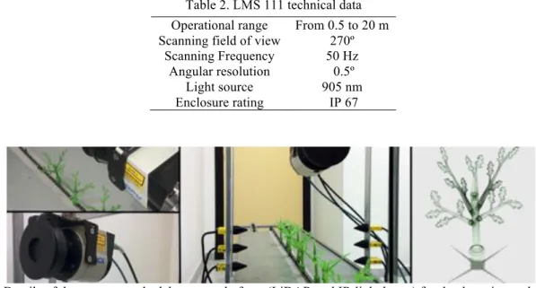
2.1.2 Laser scanner

A LiDAR laser scanner LMS111 (SICK AG, Waldkirch, Germany) was also mounted on the platform, at the top and vertically, scanning the scene below, producing a top view of the row of moving plants. Its main characteristics are summarized in Table 2. This configuration was tested on most of the measurements performed, and two other orientations of the sensor (scanning with angles of 45º and 0º) were tested to evaluate the best detection as a function of the position. The basic operating principle of this LiDAR sensor is the projection of an optical signal onto the surface of an object at a certain angle and range; by processing the corresponding reflected signal, it determines the distance to the sensor. The LiDAR sensor was interfaced to a computer through an RJ45 Ethernet port for data transfer. The vertical LiDAR orientation provided the plant’s top projection while the other two scanning positions yielded the complete vertical profile of the plants. Its resolution in the direction of travel was greatly affected by the platform’s moving speed. Maintaining a constant speed being a key factor for accurate measurements. Once the point cloud was obtained by the LiDAR sensor and represented using the self-developed software, as detailed in the following section, several distance measurements were made. Additionally, detection data were taken from the LiDAR sensor were cross-analyzed with the data obtained by the IR light beam sensors.

Table 2. LMS 111 technical data Operational range From 0.5 to 20 m Scanning field of view 270º

Scanning Frequency 50 Hz Angular resolution 0.5º

Light source 905 nm Enclosure rating IP 67

Figure 1. Details of the sensors on the laboratory platform (LiDAR and IR light beam) for the detection and structure of the modular 3D plant (left).

2.2.Field tests

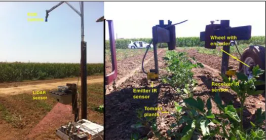
A structure coupled to the tractor's three-point hitch was designed and implemented for field trials conducted at the Western Center of Agricultural Equipment (WCAE) on the University of California, Davis campus, to carry the sensors and position them to work in field conditions (Figure 2). Field measurements with real plants were made using the same infrared photoelectric sensor (one pair of them) LiDAR for plant detection and the same position encoder described in section 2.1.. A commercial RGB action camera was placed on the top of the platform and images were taken every 3 seconds during the advance. For the field acquisition system the output signals of the sensor were connected to a bidirectional digital module (NI 9403, National Instruments Co., Austin, Texas, USA), while the position encoder was connected to a digital input module (NI 9411, National Instruments Co., Austin, Texas, USA). Both modules were integrated into a NI cRIO-9004 (NI 9411, National Instruments Co., Austin, Texas, USA), and all data were recorded using the program LabVIEW (National Instruments Co., Austin, Texas, USA).

Figure 2. Sensors mounted on the experimental platform designed for field trials in UC Davis, California 2.3.Data processing and representation

To precisely detect and properly determine the distance between plants in both laboratory and field tests, the data provided by the different sensors were analyzed and merged, allowing for discriminating between crop plants and weeds.

2.3.1 Method for the characterization of the plant by light beam sensor.

For the analysis of data obtained from the infrared light beam sensors a Matlab routine (MATLAB R2015b, MathWorks, Inc., Natick, MA, USA) was developed.

System calibration was carried out by using 11 artificial plants in laboratory test and 122 real tomato plants in field. The methodology used for the detection of tomato plants with the optical sensors was based on the following steps:

1. Selection of the values for the variables used by the program to carry out the detection:

a. pulse_distance_relation: This variable allowed us to convert the pulses generated by the position encoder into the distances travelled by the platforms. In laboratory trials the encoder was coupled to the shaft that provided motion to the 3D plants, and in field it was coupled to a ground wheel installed in the structure of the platform. The conversion factors used for the tests were 1.18 and 0.98 mm per pulse for laboratory and field respectively.

b. detection_filter: With the aim of eliminating possible erroneous detections, especially during field trials due to the interaction of leaves, branches, dust and even weeds, the data were first filtered. To do this, we proceeded to filter every detection that corresponded with a distance travelled less than 4 mm, while the sensor was active (continuous detection).

c. theoretical_plant_distance: The theoretical distance between plants in a crop line was determined during testing to be 100 mm and 380 mm for laboratory and field, respectively.

d. expected_plant_distance: Expected distance between plants in a crop line, and its theoretical value distance defined above with an error of 20%.

2. Import of raw data recorded by the sensors (encoder and existence, "1", or absence, "0", detected by the light beam sensors). The conversion factor (pulse_distance_relation) allowed us to obtain the distance in millimeters for each encoder value.

3. Data were filtered by removing all detections whose length or distance travelled, while the sensors were active, were less than the set value (detection_filter). Thus potential candidates were selected, being registered for every detection: i) the distance of the start of the detection, ii) the distance of the end of the detection iii) distance travelled during detection; iv) and mean distance during the detection, where it is considered that the stem of the plant was located.

4. Distance evaluation between the current candidate and the previous potential plant:

a. If this distance was greater than the set value (expected_plant_distance), we considered this candidate as a potential new plant to consider, registering a new matrix: the number of the plant; detections that conformed it; the location of the midpoint of the detections; the distance from the previous potential plant.

b. If this distance was less than the set value (expected_plant_distance), we added this data to previous potential candidate plant, recalculating again all potential components of this plant. For the selection of the new midpoint, the location closer to the theoretical midpoint of the new range of data was considered.

2.3.2 Method for the characterization of the plant by LiDAR+RGB data.

data and conversion from polar coordinates to Cartesian coordinates; ii) Point filtration and outlier detection to discard those points that were outside the study scene; iii) Determination of the initial and final impact points for each scan. Once point data was obtained and filtered, the resulting point cloud was visualized in an open source software (Meshlab, ISTI-CNR). This software was also used for 3D mesh creation and processing. As most points on the point cloud were part of a planar surface, point normals were automatically computed by the software. After this, given a point cloud with normals, the Ball Pivoting Algorithm (BPA) created by Bernardini et al., (1999) was used to reconstruct the surface. This algorithm starts with a seed triangle and pivots a ball with a given radius around the already formed edges until it touches another point, forming another triangle. The process continues until all reachable edges have been tried. Once the mesh was created, it was possible to measure distances directly using the measuring tools included in the Meshlab software. To help discriminate between the elements that were in the mesh, 500 images obtained by the RGB camera installed in the platform were mosaicked using Photoscan software (Agisoft Photoscan, St.Petersburg, Rusia) to obtain the texture that was merged with the mesh.

3. Results and Discussion

3.1 Laboratory tests results.

Several laboratory tests were made to properly adjust and test the sensors. As an example, Figure 3 shows the different profiles in the representations of detections, by comparing the pair of infrared sensors placed on the bottom (detecting the stems) with those placed at the middle (detecting the leaves). Figure 4 shows the positions of detected tomato stems and the estimated distance between them. In all laboratory tests the 100% stems were detected with the infrared sensor. It’s necessary to note that in laboratory conditions there are no obstacles in the crop line, a situation that is far from what we can find in the field. Figure 4 (right) shows the stem diameter measured from one of the test with an estimated average diameter of 11.2 mm and the actual value of the stem of 10 mm.

Figure 3. Signals from the light beam sensors detecting the stems (left) and leaves (right) of 11 plants in laboratory

Figure 4. Left) Positions of the stems of the 11 plants in the laboratory test. Right) Average position of the plant for a distance of 11 mm.

Results on the estimation of the plant locations made by the light beam sensors in laboratory (Figure 4) reveals that measuring the distance between plants of the same row or a treatment on the plants would be a very simple and accurate performance.

Figure 5. Left) Positions of the stems of the 11 plants in the laboratory test. Right) Average position of the plant for a distance of 11 mm.

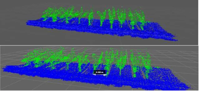
Regarding the results obtained by the LiDAR in laboratory, as mentioned in section 2.1.2, multiple scanning configurations and orientations were tested. From these tests it can be concluded that the vertical and sideway scans were those from which best point clouds were obtained and therefore plant representation and spacing measurements were more accurate. Figure 6 below show the point cloud representation of one of the scans made by the LiDAR.

Figure 6. Point cloud representation of 11 3D plants obtained by the LIDAR sensor.

3.2 Field tests results

Preliminary tests result with the infrared light beam sensors are presented in Figure 7a below. Unlike laboratory detections, in field data the determined distances between stems were more variable. This variability is mainly due to the lack of growing plants in the line caused by inaccuracies of the seeder or the presence of some weed very close to the stem of the detected plant. Figure 7b reveals that several positions for potential candidates (marked with a cross) were established, while only one potential plant should be there (marked with a circle).

(a) (b)

During the first field-test performed 41 detections occurred when there were 32 real plants growing in the seedline, this meant for this trial an error in the number of detections of 22%. However, in the trial number two 32 stem detections occurred when 34 real plants were on the line, this meant a 94% success rate. In test number three the accuracy was 98%.

Table 2. Plant detection ratio in field trials

Real plants Detected plants % Accuracy

First test 32 41 78

Second test 34 32 94

Third test 48 49 98

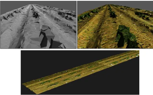
For the representation of the data obtained by the LiDAR during field trials, the team considered useful not only to represent a point cloud as was done in laboratory tests, but to generate a mesh from the point cloud and merge it with a texture generated from image mosaic. This textured mesh, besides allowing to identify and discriminate between crop plants and weeds, allowed to perform measurements on it using mesh creation software. An example meshed point-cloud is represented in the following figures below.

Figure 8. Mesh and textured mesh created from the point-cloud obtained from LiDAR sensor in field.

4. Conclusions

These initial results show that the use of an infrared sensor and a laser scanner mounted on a prototype platform represents a useful technique to accurately detect plants in a crop line and measure the distances between them. Among other achievements of this work may be mentioned:

- A successful platform sensor system for laboratory testing and field use was constructed that was able to record optical measurements (sensor and LiDAR) and position (encoder) simultaneously for a crop line.

- A high percentage (100%) of the stems were successfully detected with the infrared sensor in laboratory, while the representation of the LiDAR data would help to measure the distance between them with a low error value in the location and therefore discriminate between the crop and weeds.

- In field tests, the 90% of the plants were successfully detected, with greater variability in the distance estimation between plants. LiDAR data was successfully analyzed, providing a 3D mesh representation of the plants. A better 3D representation of row crops can help to increase the precision for decision-making to farmers, something that encourages the authors to continue working into weed detection using this technology.

Acknowledgements

Financial support received from the Spanish Ministry of Economic and Competence (Project: AGL2013-46343-R) and the Regional Government of Andalucía (Project: P12-AGR-1227) is greatly appreciated.

References

Dedousis, A. P., Godwin, R. J., O’Dogherty, M. J., Tillett, N. D., & Grundy, A. C. (2007). Inter and intra-row mechanical weed control with rotating discs. Precision Agriculture, 7, 493-498.

A.P. Papadopoulos, S. Pararajasingham. (1997). The influence of plant spacing on light interception and use in greenhouse tomato: A review. Scientia Horticulturae 69, 1-29.

Blasco, J., Aleixos, N., Roger, J., Rabatel, G., Moltó, E. (2002). Robotic weed control using machine vision. Biosystems Engineering 83, 149–157.

Christian Frasconi, Marco Fontanelli, Michele Raffaelli and Andrea Peruzzi. (2014). Design and full realization of physical weed control (PWC) automated machine within the RHEA project. Proceedings International Conference of

Agricultural Engineering. Zurich: www.eurageng.eu.

Dworak, V., Selbeck, J., Ehlert, D. (2011). Ranging sensor for vehicle-based measurement of crop stand and orchard parameters: a review. Transactions of the ASABE 54, 1497–1510.

Ehsani, M.R., Upadhyaya, S.K., Mattson, M.L. (2004). Seed location mapping using RTK-GPS. Transactions of the ASAE, Vol. 47, 909-914.

Fausto Bernardini, Joshua Mittleman, Holly Rushmeier, Claudio Silva, Gabriel Taubin. (1999). The Ball-Pivoting Algorithm for Surface Reconstruction. IEEE Transactions on visualization and computer graphics Vol 5, 349-359.

H. Sun, D.C. Slaughter, M. Pérez Ruiz, C. Gliever, S.K. Upadhyaya, R.F. Smith (2010). RTK GPS mapping of transplanted row crops. Computers and Electronics in Agriculture Volume 71, Issue 1, 32–37.

Joan R. Rosell, Jordi Llorens, Ricardo Sanz, Jaume Arnó, Manel Ribes-Dasi, Joan Masip, Alexandre Escolà, Ferran Camp, Francesc Solanelles, Felip Gràcia, Emilio Gil, Luis Val, Santiago Planas, Jordi Palacín. (2009). Obtaining the three-dimensional structure of tree orchards from remote 2D terrestrial LIDAR scanning. Agricultural and Forest Meteorology, 1505–1515.

Kyle W. Freeman, Kefyalew Girma, Daryl B. Arnall, Robert W. Mullen, Kent L. Martin, Roger K. Teal, and William R. Raun (2007). By-Plant Prediction of Corn Forage Biomass and Nitrogen Uptake at Various Growth Stages Using Remote Sensing and Plant Height. American Society of Agronomy, Journal, V99, 530–536.

Lei Li, Qin Zhang, and Danfeng Huang. (2014). A Review of Imaging Techniques for Plant Phenotyping. Sensors, 14(11).

López-Granados, F. (2011). Weed detection for site-specific weed management: Mapping and real-time approaches. Weed Research 51, 1-11.

M. S. Moran, Y. Inoue, and E. M. Barnes. (1997). Opportunities and Limitations for Image-Based Remote Sensing in Precision Crop Management. Remote Sensing 61, 319-346.

Manuel Pérez-Ruíz, David C. Slaughter, Fadi A. Fathallah, Chris J. Gliever, Brandon J. Miller. (2014). Co-robotic intra-row weed control system. Biosystems Engineering, Vol. 126, Pages 45–55.

Miguel Garrido, Dimitris Paraforos, David Reiser, Manuel Vázquez Arellano, Hans Griepentrog, Constantino Valero. (2015). 3D Maize Plant Reconstruction Based on Georeferenced Overlapping LiDAR Point Clouds. Remote Sensing, 17077-17096.

Miguel Garrido, Manuel Perez-Ruiz, Constantino Valero, Chris J.Gliever, Bradley D.Hanson, David C.Slaughter (2014). Active optical sensors for tree stem detection and classification in nurseries. Sensors 14, 10783-10803.

Miguel Garrido, Valeriano Méndez, Constantino Valero, Christian Correa, Alejandro Torre, Pilar Barreiro. (2012). Online dose optimization applied on tree volume through a laser device. First RHEA International Conference on Robotics and associated high technologies and equipment for agriculture.

Noah Fahlgren, Malia A Gehan, Ivan Baxter. «Lights, camera, action: high-throughput plant phenotyping is ready for a close-up (2015). Lights, camera, action: high-throughput plant phenotyping is ready for a close-up. Current opinion in Plant Biology, V.24 Pages 93-99.

Öner Çetina, Demet Uyganb (2008). The effect of drip line spacing, irrigation regimes and planting geometries of tomato on yield, irrigation water use efficiency and net return. Agricultural Water Management Volume 95, Issue 8, Pages 949–958.

R. Shah, W.S. Lee. (2015). An approach to a laser weeding system for elimination of in-row weeds. Precision Agriculture '15 Proceedings of the X European Conference on Precision Agriculture, 309-312.