arXiv:1504.06476v1 [math.NA] 24 Apr 2015
On Petviashvili type methods for traveling
wave computations: Acceleration techniques
J. ´
Alvarez
Department of Applied Mathematics, University of Valladolid, Paseo del Cauce 59, 47011, Valladolid, Spain.
IMUVA, Institute of Mathematics of University of Valladolid; Spain. Email: [email protected]
A. Dur´an
1Department of Applied Mathematics, University of Valladolid, Paseo de Belen 15, 47011-Valladolid, Spain.
IMUVA, Institute of Mathematics of University of Valladolid; Spain. Email: [email protected]
Abstract
In this paper a family of fixed point algorithms, generalizing the Petviashvili method, is considered. A previous work studied the convergence of the methods. Presented here is a second part of the analysis, concerning the introduction of some accelera-tion techniques into the iterative procedures. The purpose of the research is two-fold: one is improving the performance of the methods in case of convergence and the sec-ond one is widening their application when generating traveling waves in nonlinear dispersive wave equations, transforming some divergent into convergent cases. Two families of acceleration techniques are considered: the vector extrapolation meth-ods and the Anderson acceleration methmeth-ods. A comparative study through several numerical experiments is carried out.
Key words: Petviashvili type methods, traveling wave generation, iterative methods for nonlinear systems, orbital convergence, acceleration techniques, vector extrapolation methods, Anderson acceleration
MSC2010: 65H10, 65M99, 35C99, 35C07, 76B25
1 Introduction
In a previous paper [3], a family of fixed-point algorithms for the numerical approximation of nonlinear systems of the form
Lu=N(u), u∈Rm, m >1, (1)
was introduced. In (1),Lis a nonsingularm×mreal matrix andN :Rm →Rm
is an homogeneous function with degree p,|p|>1 (this means that N(λu) =
λpN(u)). Among other applications, systems of this form are very typical in
the numerical generation of traveling waves and ground states in water wave problems and nonlinear optics. For the numerical approximation to solutions of (1), the use of the classical fixed-point algorithm is not suitable. This is due
to the fact that ifu∗
is a solution and S =L−1
N′
(u∗
) stands for the iteration
matrix at u∗
, then, since N is homogeneous of degree p then N′
(u∗
)u∗
=
pN(u∗
) and therefore
Su∗
=L−1
N′
(u∗
)u∗
=pL−1
N(u∗
) =pu∗
,
that is, p is an eigenvalue of S with magnitude above one. This makes the
iteration not convergent in general.
As an alternative and based on the Petviashvili method, [56,55,46,47], the following fixed-point algorithms were considered in [3]:
Lun+1 =s(un)N(un), n = 0,1, . . . , (2)
from u0 6= 0 and where s : Rm → R is a C1 function satisfying the following
properties:
(P1) A set of fixed points of the iteration operator
F(x) = s(x)L−1
N(x), (3)
coincides with a set of fixed points of (1). This means that: (a) if u∗
is a
solution of (1) thens(u∗
) = 1; (b) inversely, if the sequence{un}n, generated
by (2), converges to somey, thens(y) = 1 (and, consequently,yis a solution
of (1)).
(P2) s is homogeneous with degreeq such that|p+q|<1.
The function s is called the stabilizing factor of the method, inheriting the
s(x) = hLx, xi
hN(x), xi
!γ
, q=γ(1−p), (4)
The first part of the work, carried out in [3] (see also [5]), analyzed the conver-gence of (2). The main conclusion was that, compared to the classical fixed-point algorithm, the stabilizing factor acts like a filter of the spectrum of the
matrix S in the sense that:
• The eigenvalue λ=pofS is transformed to the eigenvalueλ=p+q of the
iteration matrix F′
(u∗
) of (3).
• The rest of the spectrum of F′
(u∗
) is included into the spectrum of S.
Thus, the convergence of (2) depends of the spectrum of S different from p.
From these conclusions, several results of convergence can be derived, see [3] for details.
The motivation of this paper is two-fold. First, several numerical experiments in the literature show that the Petviashvili type algorithms are in sometimes computationally slower than other alternatives. In order to continue to bene-fit from the easy implementation (one of the advantages of the methods) the algorithms should improve their performance with the inclusion of some ac-celeration technique. A further motivation comes from the known mechanism of some extrapolation methods, [64], to transform divergent into convergent cases. The application of this property to these Petviashvili type methods may extend their use to compute traveling waves under more demanding con-ditions, for example in two dimensions or/and in case of highly oscillatory waves.
The literature on acceleration techniques is very rich with many different fam-ilies and strategies, [64,22]. This paper will be focused on two types of pro-cedures: the vector extrapolation methods, [22,70,41,20,66] and the Anderson mixing, [6,75,53,34]. We think that the first one is the most widely studied group; in particular, known convergence results for some of these methods will serve us to justify several examples of transformation from divergence to convergence when generating traveling waves iteratively. The second family accelerates the convergence by introducing the strategy of minimization of the residual in some norms at each step. They have been revealed efficient in, for example, electronic structure computations, [6,58] (see also [53,75] and refer-ences therein) and, to our knowledge, this is the first time they are applied to the numerical generation of traveling waves.
of the waves as an attempt to give some guidelines of application. In this sense, the paper provides several conclusions to be emphasized:
• The use of acceleration techniques is highly recommended here since it
im-proves the performance in general and allows to extend the application of the methods to computationally harder situations, with especial emphasis on two-dimensional simulations and highly oscillatory wave generation.
• By comparing the two families of acceleration techniques considered in this
study, the vector extrapolation methods are in general more competitive for these problems compared to the Anderson acceleration methods. Among the vector extrapolation methods, the polynomial methods provide a better performance in general (some exceptions can be seen in the experiments below).
• The main drawback of the Anderson acceleration methods concerns the
nu-merical treatment of the associated minimization problem, since most of the difficulties come from ill-conditioning. This might be improved by including suitable preconditioning techniques (here the methods were implemented in a standard way, [75,53,34]). However, it is remarkable that when the Ander-son acceleration methods work, their performance is in general comparable to that of some vector extrapolation methods.
The structure of the paper is as follows. Section 2 is devoted to a description of the two families of acceleration techniques considered in this study. This also includes some comments on the implementation and convergence results. The application of both techniques to the methods (2) is studied in Section 3 through a plethora of numerical experiments involving the computation of different types of traveling waves: ground states, classical and generalized soli-tary waves as well as periodic traveling waves. The numerical study will be focused on the two main motivations of the paper: the improvement of the efficiency and the extension of application of the methods to computationally harder problems and where the iteration is initially not convergent. Finally, Section 4 completes the computational study with some illustrations of the application of the acceleration to the extended versions of the algorithms (2), treated in [4] and suitable when the nonlinearity in (1) contains several homo-geneous terms with different degree. Some concluding remarks are in Section 5.
2 Acceleration techniques
efficiency. Furthermore, as in the case of the classical algorithm, [70], some cases of divergence will be transformed to convergent iterations.
This section introduces two families of acceleration techniques: the vector extrapolation methods (VEM from now on) and the Anderson acceleration methods (AAM). We will include a description of the schemes (including some convergence results) and some comments on implementation.
2.1 Vector extrapolation methods
The first group of acceleration techniques consists of vector extrapolation methods (VEM). For a more detailed analysis and implementation of the methods see [25,35,51,70,41,20,22,64] and references therein. Here we will de-scribe the general features of the procedures and their application to (2).
Two families of VEM are typically emphasized in the literature. The first one covers the so-called polynomial methods; they include, as the most widely cited, the minimal polynomial extrapolation (MPE), the reduced rank extrap-olation (RRE) and the modified minimal polynomial extrapextrap-olation (MMPE) methods, [25,35,51,70,41,66,61]. The second family consists of the so-called
ǫ-algorithms; typical examples are the scalar and vector ǫ-algorithms and the
topologicalǫ-algorithm, [18,20,41,71]. All the methods share of course the idea
of introducing the extrapolation as a procedure to transform the original
se-quence{un}of the involved iterative process by some strategy. The polynomial
methods are usually described in terms of the transformation (k≤m)
Tk :Rm −→Rm (5)
un 7−→tn,k =un−∆Un,k
V∗
n,k∆2Un,k
+
Vnk∆un,
where
• ∆un =un+1−un,∆2un= ∆un+1−∆un. • ∆iU
n.k (i= 1,2) denotes them×k matrix of columns ∆iun, . . . ,∆iun+k−1.
• Vn,k stands for the m×k matrix of some columns v(
n) 1 , . . . , v
(n)
k withV
∗
n,k as
the adjoint matrix ofVn,k (conjugate transpose).
In (5), A+ stands for the Moore-Penrose generalized inverse of A, defined as
A+ = (A∗
A)−1
A∗
, [30,52,38]. Different choices of the vectors v(jn), j1, . . . , k
lead to the most widely used polynomial methods:
(i) Minimal polynomial extrapolation (MPE): v(jn) = ∆un+j−1, j = 1, . . . , k.
(ii) Reduced rank extrapolation (RRE):vj(n) = ∆2u
(iii) Modified minimal polynomial extrapolation (MMPE): v(jn) = vj, j =
1, . . . , k, for arbitrary, fixed, linearly independent vectors v1, . . . vk ∈Rm.
The formulation of the VEM may follow an alternative approach, [66,70]. The transformation (5) can be computed in the form
tn.k = k
X
j=0
γjun+j, k
X
j=0
γj = 1, (6)
where the coefficients γj are obtained from the resolution (in some sense) of
overdetermined, inconsistent systems
k−1
X
i=0
diwn+i =wen, (7)
for some vectors wj,wej ∈ Rm. Different methods emerge by combining
dif-ferent choices of the norm where the residual vector Pk−1
i=0 diwn+1 = wen is
minimized with suitable vectors wj,wej ∈ Rm. Thus, for example, assuming
k < m, we have:
• RRE is obtained by writing (6) in the form
tn.k =un− k−1
X
j=0
βj∆un+j,
where the βj solve (7) with wj = ∆2uj,wej = ∆uj and the Euclidean norm
with equal weights is used.
• MPE is obtained by using (6) with
γj = cj
Pk i=0ci
,≤0≤j ≤k,
where ck = 1 and the cj,0 ≤ j ≤ k −1 solve (7) with wj = ∆uj,wej =
−∆uj+k in the sense of minimization with the Euclidean norm with equal
weights.
• MMPE is obtained from (6) but where instead of (7) a system of the form
k−1
X
i=0
diQj(wn+i) = Qj(wen), j = 1, . . . , k, (8)
is used. In (8)Qj(y) =hej, yi=yj, being y= (y1, . . . , ym)T.
These formulations can be unified by a representation with determinants,
tn,k =
where theui,j are scalars that depend on the extrapolation method and where
the expansion of (10) is in the sense
D(σ0, . . . , σk) = k
X
i=0
σiNi, (11)
with Ni the cofactor of σi in the first row. Thus in the case of the numerator
in (9), formula (11) is a vector, while in the case of the denominator in (9), formula (11) is a scalar. (See [23] for the interpretation in terms of the Schur complement of a matrix.) The three previously mentioned polynomial methods
correspond to the following choices ofui,j:
• MPE:ui,j =h∆un+i,∆un+ji. • RRE:ui,j =h∆2un+i,∆un+ji.
• MMPE: ui,j =hei+1,∆un+ji, where e1, . . . ek are linearly independent
vec-tors inRm.
A second family of VEM is called theǫ-algorithms. A description of them may
start from the scalar ǫ-algorithm of Wynn, [77,79]. This scalar extrapolation
method can be derived from the representation (9), (10) (in the scalar case) with ui,j = ∆un+i+j, i = 0, . . . , k−1;j = 0, . . . , k (which are scalars in the
scalar case). The corresponding ratio of determinants
tn,k =ek(un) =
D(un, un+1, . . . , un+k)
D(1,1, . . . ,1) , (12)
is called the classical e- (or Shanks Schmidt SS) transform, [67,68,76]. This
ratio can be evaluated recursively for increasing k and n without the
ǫ(−n1)= 0, ǫ
k constant. Thus, from (12), formulas (13), (14) compute each entry of a
triangular array in terms of the previous entries.
The extension of the scalar ǫ-algorithm to the vectorial case was carried out
by Brezinski, [19], and Wynn, [78,37], by using different definitions of ‘inverse’ of a vector, see [70]. Wynn suggests to consider the transpose of the Moore-Penrose generalized inverse of a vector,
w−1
= w
||w||2, (15)
leading to the vectorǫ-algorithm (VEA), whose formulas are of the form (13),
(14) where the scalars are substituted by vectors and (14) makes use of (15).
This implies that the e-transform (12) is understood in the above described
vectorial sense. This is called the generalized Shanks Schmidt (GSS) transform,
[18]. On the other hand, Brezinski defines the inverse of pair of vectors (v, w)
such thathv, wi 6= 0 as the pair of vectors (w−1
is called the inverse of v with respect to w and viceversa. This
definition leads to the so-called Topological ǫ-algorithm (TEA), when an
ar-bitrary vector y is fixed and the inverses of ∆ǫ(2nk) and ∆ǫ
(n)
2k+1 are considered
with respect toy, that is
The recursive formulas are
ǫ(−n1)= 0, ǫ
ǫ(2nk)=ek(un), ǫ(
For an efficient implementation of (16) see [71]. Thus (TEA) corresponds to take ui,j =Q(un+i+j) =hy, un+i+ji in (9), (10).
The mechanism of working of the VEM can be described as follows, see [66,70,64] for details. One starts from assuming an asymptotic expression for
the sequence un of the form
un≡u+
expansion (17) can be generalized by considering, instead of constant vectors
wj, polynomialsPj(n) in n with vector coefficients of the form
pj ≥pj+1, [65]. For simplicity, the description below will make use of (17).
The asymptotic expansion (17) is considered in a general vector space (finite or infinite dimensional) where the iteration is defined. It is understood in the
sense that any truncation differs fromun in less than some power of the next
λ. This means that for any positive integer N there are K >0 and a positive
integer n0 that only depend on N such that for every n≥n0
In particular, the case N = 1 allows to identify u as limit or anti-limit of the
sequence un, according to the size of λ1. (That is, if |λ1|<1 then limn→∞un
exists and equals u. If |λ1|>1 then limn→∞un does not exist and u is called
the anti-limit of the sequence un.) Under these conditions, several results of
convergence for MPE, RRE, MMPE and TEA are obtained in the literature, [66,70] and references therein. For these methods, one can find an extrapolation
step κ such that
The estimate (19) may explain the convergent behaviour of the extrapolation
in some cases. If the λ’s are identified as the eigenvalues of the linearization
operator of the iteration at the limit (or anti-limit)u, then the extrapolation
has the effect of translating the behaviour of the iteration to an eigenvalue
λκ+1 that may be into the unit disk, even if the previous ones are out of it.
Hence, u may be anti-limit for the original iteration and the extrapolation
converges to it. These results are extended to the defective linear case with more general polynomials (18) in [65].
The integerκis related to the concept of minimal polynomialP(λ) of a matrix
A with respect to a vectorv, [39,41,70]; this is the unique polynomial of least
degree such that
P(A)v = 0.
Thus in the case of linear iteration with matrixA, κis taken to be the degree
of the minimal polynomial of A with respect to the first iteration u0. In the
case of a nonlinear system written in fixed point form
x=F(x), (20)
then κ is theoretically defined as the degree of the minimal polynomial of
A=F′
(u∗
) with respect tou0, where u∗ is a solution of (20). In contrast with
the linear case, there is no way to determineκin advance for the nonlinear case.
This forces to consider several strategies for the choice and the corresponding implementation, see the discussion in [70] and the comments here below.
We also mention that in the linear case, the extrapolation methods MPE and RRE are mathematically equivalent to the method of Arnoldi, [59], and the GMRES, [60], respectively, see [62], while the MMPE is mathematically equivalent to the Hessenberg method, [66] and TEA to the method of Lanczos, [48], see [62,41].
Efficient and stable implementation of the RRE, MPE and MMPE methods by using QR and LU factorizations can be seen in [63,40]. For the case of TEA, see [71] and [21,61] for VEA. The implementation is usually carried out in a cycling mode. A cycle of the iteration is performed by the following steps
: consider a method (2) with a stabilizing factors satisfying (P1), (P2). Given
u0 6= 0 and a width of extrapolation mw ≥ 1, for l = 0,1, . . ., the advance
l 7→l+ 1 is:
(A) Set t0 =ul and compute mw steps of the fixed-point algorithm:
Ltn+1 =s(tn)N(tn), n = 0, . . . mw−1.
(B) Compute the extrapolation steps (9) with any of the methods described
(C) Set ul+1 =tmw,l, t0 =ul+1 and go to step (A).
The cycle (A)-(B)-(C) is repeated until the error (residual or between two consecutive iterations) is below a prefixed tolerance, a maximum number of iterations is attained or the discrepancy between the stabilizing factor at the iterations and one is below a prefixed tolerance.
The width of extrapolationmwdepends on the choice of the technique: mw=
κ+1 for MPE, RRE or MMPE andmw= 2κfor VEA or TEA, [70]. Sinceκis
generally unknown, some strategy for the implementation must be adopted. In practice, as discussed in [70], the methods are implemented with some (small)
values ofmwand take that with the best performance. It may be also different
for each cycle, although quadratic convergence is not expected ifκis too small.
This choice of κ will be computationally studied in some examples in Section
3.
The hypotheses for the expansion (17) include the conditions λj 6= 1 ∀j. In
many problems for traveling wave generation, λ = 1 appears as eigenvalue
of the iterative technique (of fixed point type) although under especial cir-cumstances that allow to extend the convergence results in some sense. This especial situation is related to the presence of symmetries in the equations for traveling waves. In order to extend the results of convergence to this case, one has to consider the orbits by the symmetry group of the equations and interpret the convergence in the orbital sense, that is a convergence for the orbits. The description of this orbital convergence can be seen in [3].
Finally, local quadratic convergence is proved in [70] (see also [49,41,39,73]) for the four methods and VEA for a general nonlinear system (20) and under
the following hypotheses on F:
• The Jacobian matrixF′
(u∗
) does not have λ= 1 as eigenvalue.
• kis the degree of the minimal polynomial of F′
(u∗
) with respect tou0−u∗.
• the algorithm is implemented in the cycling mode whereκ is chosen in the
i-th cycle as the degree of the minimal polynomial of F′
(u∗
) with respect toti−1 −u
∗
.
This result can be extended to the case whereF admits aν-parameter (ν ≥1)
group of symmetries and, consequently, λ = 1 is an eigenvalue of F′
(u∗
2.2 Anderson acceleration methods
A second family of acceleration techniques considered here is the so-called Anderson family or Anderson mixing, [6]. It is widely used in electronic struc-ture computations and only recently it has been analyzed in a more general context, [75,53,82]. (To our knowledge, this is the first time that AAM are applied to accelerate traveling wave computations.) The main goal of the ap-proach consists of combining the iteration with a minimization problem for the residual at each step. For linear problems, this technique is essentially equivalent to the GMRES method, [60,30,38]. The stages for an iteration step
are as follows: Given u0 6= 0, nw≥1, set Lu1 =s(u0)N(u0). For k = 1,2, . . .
The resolution of the optimization problem (21) is the source of the additional computational work of the acceleration. One way to reduce this extra effort is the so-called multisecant updating [34,36]. (This also clarifies the connection with quasi-Newton methods.) This technique consists of writing the problem in an equivalent form
min
γ=(γ0,...,γnk)
||f − Fkγ||,Fk = (∆fk−nk, . . . ,∆fk−1),∆fi =fi+1−fi, (22)
but with a more direct resolution, and determining the acceleration from it. The general step becomes:
As mentioned in [75], if Fkis full-rank, the solution of the minimization
prob-lem can be written as γ(k) = (FT
kFk)
−1 FT
kfk and the Anderson acceleration
has the alternative form
Luk+1=Luk−Gkfk,
Gk=−I + (Hk+Fk)(FkTFk)
−1 FT
k, Hk = (∆uk−mk, . . . ,∆uk−1),
∆ui =ui+1−ui. (23)
(Note that Gk can be viewed as an approximate inverse of the Jacobian of
Lx−N(x)). The formulation (23) motivates the generalization of the Anderson
mixing, [34]. This is performed replacing (FT
kFk)
−1
Fk in (23) by some Vk ∈
Rn×m satisfying
VkTFk =I,
and (23) becomes
Luk+1=Lxk−Gekfk,
e
Gk=−I + (Hk+Fk)VkT, Hk = (∆uk−mk, . . . ,∆uk−1). (24)
The resulting methods are collected in the so-called Anderson’s family, [75,34]. Two particular members are emphasized: the Type-I method (denoted by
AA-I from now on), which corresponds to Vk = (HkTFk)−1Hk in (24) and Type-II
method (or AA-II), which is the original Anderson mixing (23).
To our knowledge, some convergence results can be seen in [75,57,72]. In [75] the authors identify some Anderson methods for linear problems and in some sense with the GMRES method and the Arnoldi (FOM) method; some conver-gence results can be derived from this identification. In [57] the equivalence with GMRES for linear problems is completely characterized. Finally, [72] gives some proofs of convergence of the Anderson acceleration when applied
to contractive mappings: q-linear convergence of the residual for linear
prob-lems under certain conditions when nw= 1 and local r-linear convergence in
the nonlinear case. (These types of convergence are defined in the paper.)
On the other hand, as observed in [75], the implementation of AAM should be carried out by attending to three main points: a convenient formulation of the minimization problem (21), a numerical method for its efficient
resolu-tion and, finally, the parameter nw, which plays a similar role to that of the
extrapolation width mw in the VEM. In our computations below, we have
followed the treatment described in [75]. This is based on the use of the
un-constrained form (22) and its numerical resolution with QR decomposition.
references cited there. (According to our results below, the use of alternative preconditioning techniques might be recommendable in some cases.) As far as
the choice of nw is concerned, a similar strategy to that of mw will be used,
since our experiments, [75], suggest that nw(asmw) strongly depends on the
problem under study and large values are not recommended. Finally the codes
are implemented by retaining the definition of nk = min{nw, k} since other
alternatives, [82], did not improve the results in a relevant way.
3 Numerical comparisons
Presented here is a comparative study on the use of VEM and AAM as accel-eration techniques from the Petviashvili type methods (2) in traveling wave computations. The comparison is organized according to two main points: the type of traveling wave to be generated and the elements of each family of methods to be used for the generation. The first point includes the following case studies:
(1) Classical solitary waves, generalized solitary waves and periodic traveling waves of the four-parameter Boussinesq system, [11,12].
(2) Localized ground state solutions of NLS type equations, [81,80].
(3) Highly oscillatory solitary waves of the one- and two-dimensional Ben-jamin equation, [7,8,9,43,44,45].
This plethora of waves attempts to discuss and overcome different computa-tional difficulties and with the aim of establishing as more general conclusions as possible. As for the second point, each family of techniques has been rep-resented by the following methods:
• MPE and RRE standing for polynomial extrapolation methods.
• VEA and TEA standing forǫ algorithms.
• AA-I and AA-II standing for the AAM.
For simplicity, the acceleration will be applied to the Petviashvili method (2),
(4) with γ = p/(p−1). Due to the similar behaviour of the methods of the
family (2), illustrated in [3], the conclusions from the corresponding results can reasonable serve when the Petviashvili method is substituted by any of (2).
the discretization leads to a nonlinear system of algebraic equations for the approximate values of the profile at the collocation points or for the discrete Fourier coefficients of the approximation. This system is iteratively solved with the classical Petviashvili method (2), (4) along with the selected acceleration technique. This will be described in each equation considered below.
Several stopping criteria for the iterations are implemented:
• A maximum number of iterations.
• The iteration stops when one of the following quantities are below a prefixed,
small toleranceT OL:
(i) The difference in Euclidean norm between two consecutive iterations
En =||un+1−un||, n= 0,1, . . .
(ii) The residual error (also in Euclidean norm)
RESn=||Lun−N(un)||, n = 0,1, . . . (25)
(iii) The discrepancy between the stabilizing factor and (in case of conver-gence) its limit one
SF En=|s(un)−1|, n = 0,1, . . . (26)
The numerical experiments that form the comparative study are of different type:
• For several values ofκ (in the case of VEM) and nw (in the case of AAM)
we have computed the number of iterations required by each method to achieve a residual error below the prefixed tolerance. This allows to compare some performance of the methods between the two families, among different techniques within a same family and indeed with the Petviashvili method without acceleration.
• Some eigenvalues of the iteration matrices for the classical fixed point
al-gorithm and the Petviashvili method have been computed (with the corre-sponding standard MATLAB function) in order to explain the behaviour of the second one, [3] and how the acceleration eventually changes it.
• The form of the approximate profiles and some experiments to check their
accuracy are also displayed.
3.1 Traveling wave solutions of Boussinesq systems
ηt+ux+ (ηu)x+auxxx−bηxxt= 0, (27)
alternatives to model the bidirectional propagation of the irrotational free sur-face flow of an incompressible, inviscid fluid in a uniform horizontal channel under the effects of gravity when the surface tension and cross-channel
varia-tions of the fluid are assumed to be negligible. If h0 denotes the undisturbed
water depth, then η(x, t) stands for the deviation of the free surface from h0
at the point x and time t, while u(x, t) is the horizontal velocity of the fluid
at x and at the height y = θh0 (where y = 0 corresponds to the channel
bottom) at time t. For the derivation of (27) from the two-dimensional Euler
equations and the mathematical theory see [11,12]. For the modification of (28) to include the influence of surface tension see [29,27,28].
The Boussinesq system (27) admits different types of traveling wave solutions. First, being an approximation to the corresponding two-dimensional Euler equations in the theory of surface waves, it is expected to have classical solitary wave solutions. They are solutions of the initial value problem of (27) of smooth
traveling wave formη=η(x−cst), u=u(x−cst) with some speed cs >0 and
The problems of existence, asymptotic decay and stability of solutions of (29)
have been analyzed in many references and for particular values of a, b, c, d,
see [33] and references therein. Furthermore, in the same reference, linearly well-posed systems (29) may be studied as a first order ode system and, based on normal form theory, a discussion on the values of the parameters leading to Boussinesq systems admitting solitary wave solutions with speed
cs > 1 is established. According to it, two classes of systems can be
distin-guished. The first one admits classical (in the sense above defined) solitary
wave solutions. This group contains the Bona-Smith system (a = 0, b = d =
(3θ2 −1)/6, c = (2−3θ2)/3,2/3 < θ2 < 1), [15], or the BBM-BBM system
(a=c= 0, b=d= 1/6), [10]. (The classical Boussinesq system, which
the general discussion of [33] and has been studied separately, [54].) A second class of Boussinesq systems admits generalized solitary wave solutions, that is traveling wave profiles which are not homoclinic to zero at infinity but to small
amplitude periodic waves, [50]. The KdV-KdV system (a=c >0, b=d= 0),
[13,14], is an example of this second group.
Finally, the existence of periodic traveling wave solutions of (27) is studied in [26] by applying topological degree theory for positive operator to the
corre-sponding periodic initial value problem posed on an interval (−l, l) and some
cnoidal wave solutions of the BBM-BBM system are computed. A smooth
periodic traveling wave solution η = η(x.cst), u = u(x.cst) with some speed
cs >0 must satisfy the ode system
for some real constants K1, K2. These are related to the period parameter l.
The resolution of (30) involves a modified system for which these constants of integration are set to zero, [26]. This is briefly described as follows. One
first searches for constant solutions η=C1, u=C2 of (30). This leads to the
which can be solved as a cubic equation for C2:
C3
This strategy will be considered in the numerical generation of the profiles in (30): the system (33) wil be discretized to compute approximations to the
In order to generate numerically classical and generalized solitary wave solu-tions of (27) the corresponding periodic value problem of (29) on a long enough
interval (−l, l) is discretized with a Fourier collocation method leading to a
discrete system of the form
Dis the pseudospectral differentiation matrix, [17,24],Im is them×midentity
matrix and the nonlinear term N, which is homogeneous of degree p = 2,
involves Hadamard products. In the case of periodic traveling waves and as was mentioned above, system (34) will be substituted in the implementation by
The methods (2) along with the corresponding acceleration technique are then applied to the discrete systems (34) and (35). The implementation is performed in the Fourier space; for example (34) becomes
m/2. (For simplicity, we assume that m = 2s for some s > 1.) Alternatively,
where ∗ denotes periodic convolution and if ω = exp(−2πi/m), the vectors
Ah, Bh, Ch have discrete Fourier coefficients
(Ach)p =
In order to explain the behaviour of the iteration, the size of the eigenvalues of the iteration matrix will be relevant in the numerical study. In this case, the corresponding iteration matrix of the classical fixed point iteration at a
solution u∗
(where diag(v) stands for the diagonal matrix with diagonal entries given
by the components of v ∈ Rm). Some information on the spectrum of S is
known. We already have the eigenvalue λ= 2, corresponding to the degree of
homogeneity of the nonlinear part, withu∗
= (η∗
h, u
∗
h) as an eigenvector. Also,
the application of D to (34) leads to
csDη
eigenvector. This corresponds to the ‘translational’ invariance of (27).
Three particular systems of (27) will be taken to illustrate the numerical gen-eration of traveling waves. The first one is the classical Boussinesq system
ηt+ux+ (ηu)x= 0,
ut+ηx+uux−
1
3uxxt= 0. (36)
which is known to have classical solitary wave solutions, [54]. The second one
is the so-called KdV-KdV system (a=c= 1/6, b=d= 0)
ηt+ux+ (ηu)x+
1
6uxxx= 0,
ut+ηx+uux+
1
6ηxxx= 0, (37)
that admits generalized solitary wave solutions, [13,14]. Finally, in order to illustrate the numerical generation of periodic traveling waves, the BBM-BBM
system (a=c= 0, b=d= 1/6),
ηt+ux+ (ηu)x−
1
6ηxxt= 0,
ut+ηx+uux−
1
6uxxt= 0, (38)
will be taken, [26].
3.1.1 Numerical generation of classical solitary waves of (36)
In the case of system (36) a first experiment of comparison of the acceleration
techniques has been made by takingcs= 1.3 and a hyperbolic secant profile as
initial iteration withl = 64 andm= 1024 collocation points. The Petviashvili
method (2), (4) withγ = 2 was first run, generating approximateηand u
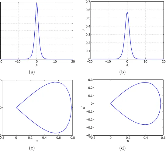
pro-files as shown in Figures 1(a) and (b) while Figures 1(c) and (d) stand for the corresponding phase portraits of the approximate profiles in (a) and (b). (They show the classical character of the solitary waves, represented as homoclinic to zero orbits with exponential decay, [54]. ) The accuracy of the iteration is checked in Figure 2. Figure 2(a) illustrates the convergence of the sequence
sn =s(ηn, un) of stabilizing factors, computed with the corresponding formula
(4) and the optimal value γ = 2. The discrepancy (26) is below the tolerance
T OL= 10−13
inn = 62 iterations, while the first residual error belowT OLis
9.092489E−14 at n= 76. (This also happens in the rest of the experiments:
when the procedure is convergent, the error |1−sn| achieves the tolerance
−200 −10 0 10 20
Fig. 1. Approximate profiles generated by the Petviashvili method (2), (4) for (36) withcs= 1.3: (a) η, (b)u; (c) Phase portrait ofη, (d) Phase portrait ofu.
Iteration matrixS(ηf, uf) Iteration matrixF′(ηf, uf) 1.999999E + 00 9.999999E −01
9.999999E −01 6.763242E −01
6.763242E −01 5.411229E −01
5.411229E −01 4.820667E −01
4.820667E −01 4.567337E −01
4.567337E −01 4.465122E −01 Table 1
Classical solitary wave generation of (36) . Six largest magnitude eigenvalues of the approximated iteration matrixS =L−1
N′
(ηf, uf) (first column) and of the iteration matrix F′
(ηf, uf), generated by the Petviashvili method (2), (4) with γ = 2, both evaluated at the last computed iterate (ηf, uf).
computed iterate (ηf, uf). The first column reveals the dominant eigenvalues
λ1 = 2, λ2 = 1, both simple, while the rest is below one. The filtering effect of
the Petviashvili method, [3], is observed in the second column; the dominant
eigenvalue is filtered to zero (recall thatγ = 2) and the rest is preserved. Since
λ2 = 1 corresponds to the translational symmetry of (27), this guarantees the
local convergence of the method (also in the orbital sense mentioned above).
The improvement of the performance of the Petviashvili method with several acceleration techniques is now computationally analyzed. A first point to study
is the choice of the parametersκ(for the VEM) andnw (for the AAM). Table
2 shows, for values ofκbetween one and ten, the number of iterations required
by MPE, RRE, VEA and TEA to achieve a residual error belowT OL= 10−13
. (The residual error, corresponding to the last iteration is in parenthesis for each computation.) From these results, the following comments can be made:
(a) For κ ≥ 2, all the methods improve the performance of the Petviashvili
method without acceleration (cf. Figure 2(b)). The reduction in the
num-ber of iterations varies in a range 50−70%.
(b) In general, polynomial methods (MPE and RRE, which essentially
be-haves in an equivalent way) are more efficient than ǫ-algorithms (with
VEA slightly better than TEA). In the best cases, the improvement is about 70% in the case of MPE and RRE and RRE, about 65% with respect to VEA and about 54% in the case of TEA. (However, one has to take into account that the cycle in the case of polynomial methods is
mw=κ+ 1 and in the case ofǫ-algorithms is mw= 2κ; cf. Figure 3.)
In the case of the AAM, the corresponding results are in Table 3. Now, the role
of the parameter κ (or mw) is played by nw. The results show that the
κ MPE(κ) RRE(κ) VEA(κ) TEA(κ)
1 269 99 631 408
(8.9136E−14) (9.1312E−14) (9.7920E−14) (7.3356E−14)
2 64 48 43 43
(7.4794E−14) (8.3903E−14) (7.7841E−14) (8.1979E−14)
3 43 43 38 42
(7.5001E−14) (8.0682E−14) (7.7395E−14) (9.6255E−14)
4 33 33 33 37
(7.9601E−14) (8.2823E−14) (7.7824E−14) (8.0527E−14)
5 28 28 31 39
(8.5285E−14) (9.8557E−14) (8.7444E−14) (9.3163E−14)
6 26 26 29 35
(8.3589E−14) (7.7189E−14) (7.3281E−14) (7.9462E−14)
7 27 27 33 35
(8.6403E−14) (8.1151E−14) (7.2215E−14) (8.4479E−14)
8 27 25 29 37
(9.7379E−14) (8.0842E−14) (7.3955E−14) (7.4142E−14)
9 23 24 30 41
(9.5276E−14) (8.3798E−14) (8.7013E−14) (7.2068E−14)
10 25 25 27 35
(7.6433E−14) (8.3980E−14) (9.3658E−14) (8.5795E−14) Table 2
Classical solitary wave generation of (36) . Number of iterations required by MPE, RRE, VEA and TEA as function of κ to achieve a residual error below T OL = 10−13
. The residual error at the last computed iterate is in parenthesis. Without acceleration, the Petviashvili method (2), (4) with γ = 2 requiresn= 76 iterations with a residual error 9.0925E−14.
with nw = 8 in the case of AA-I and nw = 9 for the AA-II. On the other
hand, as mentioned in [53,75], the value ofnw cannot be too large, because of
ill-conditioning. In this example, this was observed for AA-I whennw = 9,10.
(The corresponding results in Table 3 were obtained by using standard precon-ditioning.) Finally, compared to the Petviashvili method without acceleration,
the reduction in the number of iterations is in range of 50−80%.
nw AA-I(nw) AA-II(nw)
1 38(8.4014E −14) 35(4.8504E −14)
2 28(4.9835E −14) 26(5.6978E −14)
3 28(5.5678E −14) 25(6.2897E −14)
4 27(3.8773E −14) 22(1.4624E −14)
5 22(4.4004E −14) 20(6.5530E −14)
6 21(7.9925E −14) 21(2.4615E −14)
7 21(2.3111E −14) 20(5.3227E −14)
8 20(8.0666E −14) 20(2.7701E −14)
9 20(4.5873E −14) 19(9.6556E −14)
10 20(2.7208E −14) 19(6.8255E −14) Table 3
Classical solitary wave generation of (36) . Number of iterations required by AA-I and AA-II as function of nw to achieve a residual error below T OL= 10−13
. The residual error at the last computed iterate is in parenthesis. Without acceleration, the Petviashvili method (2), (4) withγ= 2 requiresn= 76 iterations with a residual error 9.0925E−14.
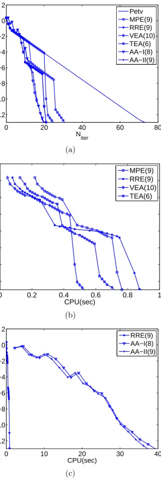
example, we have measured the performance by computing the residual error as function of the number of iterations (i. e. comparing the best results of Tables 2 and 3) and as function of the computational time. The comparison of the methods in terms of the number of iterations is illustrated in Figure 3(a). This shows, in semilogarithmic scale, the residual error as function of the number of iterations for the Petviashvili method without acceleration (solid line) and accelerated with the six selected techniques, implemented with the
values ofκandnwthat, according to Tables 2 and 3, lead to the best number of
iterations. For this example, the AA-I(8) and AA-II(9) give, for a tolerance of
T OL= 10−13
in the residual error, a slightly smaller number of iterations than the (mostly equivalent) RRE(9) and MPE(9). The initially worse performance of VEA(10) and TEA(6) is corrected after the first cycle. For example, in the case of VEA(10), after this first cycle, Figure 3(a) shows that the reduction in the residual error is the fastest.
0 20 40 60 80
Iteration matrix S(ηf, uf) Iteration matrix F′(ηf, uf) 1.999999E + 00 1.000000E + 00
1.000000E + 00 5.625613E −01
5.625613E −01 −3.525656E−01
−3.525656E−01 −3.521308E−01
−3.521308E−01 3.069304E−01 +i6.906434E−02
3.069304E−01 +i6.906434E−02 3.069304E−01−i6.906434E−02 Table 4
Generalized solitary wave generation of (37) . Six largest magnitude eigenvalues of the approximated iteration matrix S = L−1
N′
(ηf, uf) (first column) and of the iteration matrix F′
(ηf, uf), generated by the Petviashvili method (2), (4) with
γ = 2, both evaluated at the last computed iterate (ηf, uf).
explanation of it.)
3.1.2 Numerical generation of generalized solitary waves of (37)
Here we show the results concerning the generation of approximate generalized solitary waves of the KdV-KdV system (37). In this case we have considered
a speed cs = 1.3 and a Gaussian-type profile as initial guess for η and u,
with l = 64 and m = 1024 Fourier collocation points. The approximate η
and u profiles generated by the Petviashvili method (without acceleration)
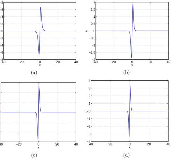
are displayed in Figures 4(a) and (b) respectively (observe the oscillatory ripples to the left and right of the main pulse), and the performance of the method (measured in terms of the convergence of the stabilizing factor and the behaviour of the residual error as function of number of iterations) is shown in Figures 4(c) and (d) respectively. The method achieves a residual error of
1.150546E−12 inn = 47 iterations and 7.859422E−14 inn = 52 iterations.
In this case, the corresponding phase portraits in Figures 5(a) and (b) show the generalized character of the waves, with orbits that are homoclinic to small amplitude periodic oscillations at infinity. The last computed iterate, corresponding to this residual error, is used to evaluate the iteration matrices
S(ηf, uf) and F′(ηf, uf) of the classical fixed point and Petviashvili method,
respectively. The associated six largest magnitude eigenvalues are shown in Table 4. (The generalized character of the computed solitary wave is also noticed by the presence of conjugate complex eigenvalues in the linearization matrix at the wave, cf. Table 1.)
−30 −20 −10 0 10 20 30
Fig. 4. Generalized solitary wave generation of (37). (a)-(b) Approximate η and u
profiles generated by the Petviashvili method (2), (4) for (37); (c) Discrepancy (26) for the stabilizing factor sn=s(ηn, un) vs number of iterations; (d) Residual error (25) vs number of iterations. (Semi-logarithm scale in both cases.)
−0.2 0 0.2 0.4 0.6 0.8
κ MPE(κ) RRE(κ) VEA(κ) TEA(κ)
1 93 64 283 67
(8.2739E−14) (9.4330E−14) (6.7393E−14) (6.5919E−14)
2 42 43 81 49
(9.3934E−14) (8.6837E−14) (6.1237E−14) (8.7121E−14)
3 37 37 38 37
(9.8740E−14) (5.6549E−14) (6.7020E−14) (7.5320E−14)
4 33 32 39 30
(7.5531E−14) (6.9363E−14) (3.6501E−14) (4.2863E−14)
5 28 28 32 30
(6.6301E−14) (7.0496E−14) (5.9777E−14) (8.5244E−14)
6 28 28 29 28
(7.8419E−14) (7.4939E−14) (3.2861E−14) (7.7335E−14)
7 27 27 32 32
(3.0803E−14) (3.2406E−14) (6.5803E−14) (4.9439E−14)
8 23 23 28 29
(9.3872E−14) (8.8601E−14) (8.0707E−14) (9.1792E−14)
9 23 23 26 27
(3.0380E−14) (3.1758E−14) (6.4506E−14) (8.0379E−14)
10 24 24 24 28
(5.8031E−14) (5.0834E−14) (7.1291E−14) (5.8663E−14) Table 5
Generalized solitary wave generation of (37) . Number of iterations required by MPE, RRE, VEA and TEA as function of κ to achieve a residual error below
T OL = 10−13
. The residual error at the last computed iterate is in parenthesis. Without acceleration, the Petviashvili method (2), (4) with γ = 2 requiresn= 52 iterations with a residual error 7.8594E−14.
in terms of the number of iterations, AAM give the best performance and amongst the VEM, the extrapolation methods MPE and RRE are (in this case
slightly) more efficient than the vectorǫ-algorithms VEA and TEA, see Figure
0 10 20 30 40 50 60
Fig. 6. Convergence results of the Petviashvili method for (37): (a) Residual error (25) as function of number of iterations for the Petviashvili method without accel-eration and for six accelaccel-eration techniques with the best parameters mw and nw
nw AA-I(nw) AA-II(nw)
1 28(7.6888E −14) 30(3.6918E −14)
2 21(3.2119E −14) 21(3.4864E −14)
3 19(4.9065E −14) 20(4.6961E −14)
4 19(2.5310E −14) 18(1.9550E −14)
5 18(5.9489E −14) 18(4.2896E −14)
6 18(2.0285E −14) 18(1.1674E −14)
7 17(5.1055E −14) 17(5.5586E −14)
8 17(2.8378E −14) 17(1.9837E −14)
9 17(7.2231E −14) 16(7.1040E −14)
10 17(2.8512E −14) 16(5.7507E −14) Table 6
Generalized solitary wave generation of (37) . Number of iterations required by AA-I and AA-AA-IAA-I as function ofnwto achieve a residual error below T OL= 10−13
. The residual error at the last computed iterate is in parenthesis. Without acceleration, the Petviashvili method (2), (4) withγ= 2 requiresn= 53 iterations with a residual error 7.8594E−14.
3.1.3 Numerical generation of periodic traveling waves of (38)
The numerical generation of periodic traveling wave solutions of the BBM-BBM system (38) will complete the study about traveling wave generation of Boussinesq systems (27). Here the initial data are similar to those of the
previous cases, although now l = 16 is taken. Once system (31) is solved,
the application of the Petviashvili type method to (35) generates, for K1 =
0.75, K2 = 1 (taken as an example) the computed profiles shown in Figure
7(a)-(b). The periodic behaviour is also observed in the corresponding phase plots, shown in Figure 7(c), (d), while the performance is illustrated in Figure 8, which corresponds to the behaviour of the residual error as function of the
number of iterations. The method attains a residual error of 9.335366E−12
inn = 572 iterations, showing the need of some acceleration technique.
This slow performance is justified by the corresponding table of eigenvalues of the linearization operators, Table 7 in this case. We observe that besides eigenvalue one (associated to the translational invariance) the next largest in magnitude eigenvalue is close to one. (As in the generalized solitary wave generation the presence of conjugate complex eigenvalues, in this case with algebraic multiplicity above one, in the spectrum of the linearization matrices is noticed.)
−15 −10 −5 0 5 10 15
Fig. 7. Numerical generation of periodic traveling waves of (38). Approximate pro-files for K1 = 0.75, K2 = 1. (a) η profile; (b) u profile; (c) η phase portrait. (d) u
Iteration matrix S(ηf, uf) Iteration matrixF′(ηf, uf) 2.000000E+ 00 1.000000E+ 00
1.000000E+ 00 −9.545242E−01
−9.545242E −01 −5.353103E−01−6.459204E−01i
−5.353103E−01−6.459204E−01i −5.353103E−01−6.459204E−01i
−5.353103E−01−6.459204E−01i −5.353103E−01 + 6.459204E−01i
−5.353103E−01 + 6.459204E−01i −5.353103E−01 + 6.459204E−01i
Table 7
Periodic traveling wave generation of (38) with K1 = 0.75, K2 = 1. Six largest
magnitude eigenvalues of the approximated iteration matrix S = L−1
N′
(ηf, uf) (first column) and of the iteration matrixF′
(ηf, uf), generated by the Petviashvili method (2), (4) withγ = 2, both evaluated at the last computed iterate (ηf, uf).
The standard comparison in performance is given in Table 8. In this case the
tolerance for the residual error was set as T OL = 10−11
. Some conclusions from it are the following:
(1) Better performance of polynomial methods compared to ǫ-algorithms.
(2) MPE and RRE are virtually equivalent, especially when κ grows. There
are more differences between VEA and TEA, but they decrease when κ
grows.
(3) For polynomial methods, the best results are obtained for largeκ(around
κ= 9) while for ǫ algorithms, it is better to take smallκ (around mw=
4,5). This implies a similar length of each cycle (width of extrapolation).
We now analyze the results corresponding to AAM by using Table 9, which evaluates the performance of AA-I and AA-II for the same example. Some conclusions from Table 9:
(1) As in some previous cases the AAM (particularly AA-II) behave better than any VEM when measuring the performance in terms of the number of iterations. However, the polynomial methods MPE and RRE are more efficient in terms of the computational time, see Figure 9.
(2) The best results of AA-II are obtained with large values of nw. The
method does not appear to be affected by ill-conditioning, contrary to
AA-I, which becomes useless from nw= 7.
3.2 Example 2. Localized ground state generation
partic-κ MPE(κ) RRE(κ) VEA(κ) TEA(κ)
1 118 278 88
(8.9607E−12) (7.1073E−12) (4.9649E−12)
2 70 81 81 81
(9.2990E−12) (6.8950E−12) (6.8161E−12) (6.8798E−12)
3 54 53 78 64
(9.4403E−12) (7.2397E−12) (4.2025E−12) (9.4892E−12)
4 47 52 55 55
(7.0369E−12) (5.3720E−12) (4.0063E−12) (7.4587E−12)
5 55 46 48 103
(4.0773E−12) (8.2635E−12) (9.7571E−12) (6.2560E−12)
6 46 44 53 79
(9.9878E−12) (5.3034E−12) (5.7135E−12) (5.4689E−12)
7 45 49 51 73
(7.4645E−12) (3.6062E−12) (9.3703E−12) (8.3118E−12)
8 45 46 53 69
(9.1401E−12) (4.3655E−12) (9.0789E−12) (4.4378E−12)
9 41 41 58 77
(9.9555E−12) (4.7100E−12) (9.8141E−12) (8.4583E−12)
10 45 45 64 64
(3.9218E−12) (4.4096E−12) (6.2339E−12) (5.0514E−12) Table 8
Periodic traveling wave generation of (38). Number of iterations required by MPE, RRE, VEA and TEA as function ofκto achieve a residual error (25) belowT OL= 10−11
. The residual error at the last computed iterate is in parenthesis. Without acceleration, the Petviashvili method (2), (4) withγ = 2 requiresn= 572 iterations with a residual error 9.3354E−12.
ular, the equation
iut+∂xxu+V(x)u+|u|2u= 0, (39)
with potential V(x) = 6sech2(x), is considered as an example, [46,80]. A
lo-calized ground state solution of (39) has the form u(x, t) = eiµtU(x), where
µ ∈ R and U(x) is assumed to be real and localized (U → 0, |x| → ∞).
nw AA-I(nw) AA-II(nw)
7 Ill-conditioned 38(2.4939E −12)
8 Ill-conditioned 36(7.2839E −12)
9 Ill-conditioned 35(8.3908E −12)
10 Ill-conditioned 37(2.6179E −12) Table 9
Periodic traveling wave generation of (38). Number of iterations required by AA-I and AA-II as function of nwto achieve a residual error (25) below T OL= 10−13
. The residual error at the last computed iterate is in parenthesis. Without accelera-tion, the Petviashvili method (2), (4) withγ = 2 requiresn= 572 iterations with a residual error 9.3354E−12.
Fig. 9. Numerical generation of periodic traveling waves of (38). Residual error (25) as function of: (a) number of iterations and (b) CPU time (in seconds) for MPE(9) and AA-II(9).
U′′
(x) +V(x)U(x)−µU(x) +|U(x)|2U(x) = 0. (40)
A discretization of (40) based on a Fourier collocation method on a sufficiently
long interval (−l, l) requires in this case the resolution of a system of the form
(1) for the approximations Uh of U at the grid points xj = −l +jh, h =
L=D2+ diag(V)−µIm, N(Uh) =−Uh.3,
where D is the pseudospectral differentiation matrix, diag(V) is the diagonal
matrix with elements Vj = V(xj), j = 0, . . . , m− 1 and Im is the m ×m
identity matrix. The nonlinearityN is homogeneous with degree three, where,
as usual, the dot stands for the Hadamard product. The discussion below is
−40 −20 0 20 40
Fig. 10. Numerical generation of localized ground states of (40). Approximate asym-metric profile. (a)µ= 1.3; (b) µ= 3.3; (c) µ= 6.3; (d) µ= 8.3. The amplitude of the waves increases withµ, while the shape is narrower.
focused on the ground state numerical generation for several values ofµ, which
provide different challenges to the iteration. For each considered value of µ,
the performance of both families of acceleration techniques has been checked.
The first results concern the numerical generation of an asymmetric solution
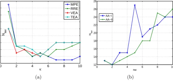
of (40) for µ = 1.3 (Figure 10(a)). Figure 11 compares the performance of
the acceleration techniques in terms of the number of iterations required to
reduce the residual error (25) below T OL = 10−12
and as function of the
ex-trapolation width parameters κ and nw. In the case of VEM, Figure 11(a),
all the techniques considered are comparable and the differences are not very
κ = 8,9 also lead to the same number of iterations, but the computational effort in CPU time is higher.) The AAM, Figure 11(b), are competitive with
VEM for small values of nw (nw = 1,2). As nw grows, the number of
iter-ations increases (in opposite way to the behaviour of VEM with respect to
κ) and the computation of the coefficients in the minimization problem
be-comes ill-conditioned. The comparison between the most efficient method of each family (MPE(7) and AA-II(2) respectively) is displayed in Figure 12. It
0 2 4 6 8 10
Fig. 11. Numerical generation of asymmetric ground state of (40) with µ = 1.3. Number of iterations required to reduce the residual error (25) belowT OL= 10−12
and as function of the extrapolation width parameters κ and nw. (a) VEM; (b) AAM.
shows the residual error as function of the number of iterations (a) and the CPU time (b) for the Petviashvili method without acceleration (solid line) and accelerated with MPE(7) and AA-II(2). In both figures, the improvement in the performance with respect to the Petviashvili method provided by the two acceleration techniques is observed, with the best results corresponding to MPE (and, in general VEM against AAM). Table 10 confirms the convergence of the Petviashvili method. It displays the six largest magnitude eigenvalues of the corresponding iteration matrix of the classical fixed-point algorithm
S = L−1
N′
(Uf), and of the Petviashvili method (3), (4) for two values of µ.
Since an analytical expression for the exact profile is not known, the matrices have been evaluated at the last computed iterate given by MPE(7). In the
case of S (first column), the dominant eigenvalue corresponds to the degree
of homogeneity p = 3, with the rest of the eigenvalues below one. The filter
action of the stabilizing factor is observed in the second column. The degree
p= 3 has been subtituted by zero (the optimal q =γ(1−p) = −p has been
taken) and the rest of the spectrum is preserved. This implies that forµ= 1.3,
the spectral radius of F′
(u∗
) is below one (second column) and this leads to the (local) convergence of the method.
numer-2 4 6 8 10 12 14
10−10
10−5
100
105
N iter
RES(n)
Petv MPE(7) AA−II(2)
(a)
0 0.2 0.4 0.6 0.8 1
10−12
10−10
10−8
10−6
10−4
10−2
100
102
CPU time
RES(n)
Petv MPE(7) AA−II(2)
(b)
Fig. 12. Numerical generation of assymetric ground state of (40) withµ= 1.3. Resid-ual error (25) as function of the number of iterations (a) and CPU time in seconds (b) for the Petviashvili method without acceleration (solid line) and accelerated with MPE(7) (circle symbols) and AA-II(2) (plus symbols).
ical generation of an asymmetric solution of (40) (see Figure 10(b)) with the Petviashvili method without acceleration is not possible in general. Table 10 (third column) shows the presence of an additional eigenvalue with magnitude
above one in the iteration matrix S of the classical fixed point algorithm. As
part of the spectrum different from the degree of homogeneity p = 3, this
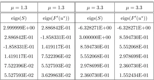
µ= 1.3 µ= 1.3 µ= 3.3 µ= 3.3
2.999999E+00 2.886842E-01 -6.328271E+00 -6.328271E+00
2.886842E-01 -1.858331E-01 3.000000E+00 8.594730E-01
-1.858331E-01 1.419117E-01 8.594730E-01 5.552068E-01
1.419117E-01 7.522396E-02 5.552068E-01 2.978699E-01
7.522396E-02 5.527593E-02 2.978699E-01 2.360730E-01
5.527593E-02 3.629863E-02 2.360730E-01 1.552434E-01 Table 10
Numerical generation of asymmetric profile of (40) with µ= 1.3 and µ = 3.3. Six largest magnitude eigenvalues of the approximated iteration matrix of the classical fixed-point methodS=L−1
N′
(Uf) (left) and of the Petviashvili method, evaluated at the last computed iterateUf obtained with MPE(7).
virtually the same performance while the ǫ-algorithms start reducing their
efficiency. (In this case, TEA does not always work in a reliable way and is not competitive against the other VEM.) As far as the AAM are concerned, Figure 13(b), both improve the performance in a similar, relevant way. They are comparable with VEM in number of iterations (Figure 14(a)) and behave better when measuring the computational time (Figure 14(b)).
0 2 4 6 8 10
Fig. 13. Numerical generation of asymmetric ground state of (40) with µ = 3.3. Number of iterations required to reduce the residual error (25) belowT OL= 10−12
and as function of the extrapolation width parameters κ and nw. (a) VEM; (b) AAM.
It may be worth considering the case µ= 6.3 because of some relevant points.
The first one is the generation of the asymmetric profile, Figure 10(c), which in general is not possible with the Petviashvili method without acceleration.
0 5 10 15 20
Fig. 14. Numerical generation of asymmetric ground state of (40) with µ = 3.3. Residual error (25) as function of the number of iterations (a) and CPU time in seconds (b) for the Petviashvili method without acceleration (solid line) and accel-erated with MPE(8) (circle symbols) and AA-II(5) (plus symbols).
in Table 11 (first and second columns). In this case, the best results of the acceleration are given by MPE and AA-I (Figure 15). The loss of performance
of the ǫ-algorithms and the improvement of AAM, observed in the previous
experiments, are confirmed here and in the experiments for µ= 8.3 (Figures
17 and 18). The comparison between MPE and AA-I, see Figures 16(a), (b), reveals, ikn the authors’ opinion, a similar performance.
2 4 6 8 10
Fig. 15. Numerical generation of asymmetric ground state of (40) with µ = 6.3. Number of iterations required to reduce the residual error (25) belowT OL= 10−12
and as function of the extrapolation width parameters κ and nw. (a) VEM; (b) AAM.
The second question with regard to the case µ = 6.3 concerns the behaviour
can-0 5 10 15 20 25 30 35
Fig. 16. Numerical generation of asymmetric ground state of (40) with µ = 6.3. Residual error (25) as function of the number of iterations (a) and CPU time in seconds (b) for the Petviashvili method without acceleration (solid line) and accel-erated with MPE(10) (circle symbols) and AA-I(5) (triangle symbols).
µ= 6.3 µ= 6.3 µ= 8.3 µ= 8.3
5.095370E+00 5.096207E+00 3.962824E+00 3.962824E+00
3.000000E+00 9.672929E-01 2.999999E+00 9.807797E-01
9.672929E-01 7.506018E-01 9.807797E-01 8.081404E-01
7.506018E-01 4.078905E-01 8.081404E-01 4.459845E-01
4.078905E-01 3.472429E-01 4.459845E-01 4.030040E-01
3.472429E-01 2.032986E-01 4.030040E-01 1.929797E-01 Table 11
Numerical generation of asymmetric profile of (40) with µ= 6.3 and µ = 8.3. Six largest magnitude eigenvalues of the approximated iteration matrix of the classical fixed-point method S = L−1
N′
(Uf) (left) and of the Petviashvili method (2), (4), evaluated at the last computed iterate Uf obtained with MPE(10).
not be convergent. However, according to the information provided by Table 12, this is locally convergent to the symmetric solution. (In this case, the
spec-tral radius of F′
(u∗
) is below one.) This profile can be indeed approximated by using acceleration techniques (and with the corresponding computational saving) but starting from a different initial iteration.
Finally, the case µ= 8.3 is also analyzed, see Figure 10(d). The main reason
we find to emphasize this case is to confirm the conclusions obtained from the
experiments with the previous values ofµ:
eigs(S) eigs(F′
(u∗
))
3.000000E+00 6.098684E-01
6.098684E-01 2.696853E-01
2.696853E-01 1.518421E-01
1.518421E-01 1.039553E-01
1.039553E-01 6.046185E-02
6.046185E-02 5.492737E-02 Table 12
Numerical generation of symmetric profile of (40) with µ = 6.3. Six largest mag-nitude eigenvalues of the approximated iteration matrix of the classical fixed-point methodS =L−1
N′
(Uf) (left) and of the Petviashvili method (2), (4), evaluated at the last computed iterateUf obtained with Petviashvili method (2), (4).
the ǫ-algorithms become less efficient asµincreases. As observed in Figure
10, the largerµthe larger and narrower the asymmetric profile is. The
com-putation becomes harder as is noticed by comparing the iterations required by the methods in Figures 11, 13, 15 and 17. One can also note the in-crement of the magnitude of the eigenvalues of the corresponding iteration matrices of the Petviashvili method in Tables 10 and 11. Therefore, under more demanding conditions, the polynomial methods give a better answer
than the ǫ-algorithms.
• Contrary to theǫ-algorithms, whose performance gets worse asµincreases,
the AAM improve their behaviour up to being comparable with polynomial methods (cf. the periodic traveling wave generation in Section 3).
Further-more, this is obtained with small values of the parameternw, thus avoiding
ill-conditioned problems.
3.3 Example 3. Solitary wave solutions of the Benjamin equation
2 4 6 8 10
Fig. 17. Numerical generation of asymmetric ground state of (40) with µ = 8.3. Number of iterations required to reduce the residual error (25) belowT OL= 10−12
and as function of the extrapolation width parameters κ and nw. (a) VEM; (b) AAM.
Fig. 18. Numerical generation of asymmetric ground state of (40) with µ = 8.3. Residual error (25) as function of the number of iterations (a) and CPU time in seconds (b) for the Petviashvili method without acceleration (solid line) and accel-erated with MPE(7) (circle symbols) and AA-II(3) (plus symbols).
3.3.1 One-dimensional Benjamin equation
A first example of the situation described above is given by the solitary wave solutions of the Benjamin equation, [7]
ut+αux+βuux−γHuxx−δuxxx= 0, (41)
whereu=u(x, t), x∈R, t≥0, α, β, γ, δare positive constants, andHdenotes
the Hilbert transform defined on the real line as
−30 −20 −10 0 10 20 30 −0.5
0 0.5 1 1.5 2
x
u
Fig. 19. Numerical generation of symmetric ground state of (40) with µ = 6.3. Approximate profile with Petviashvili method without acceleration.
or through its Fourier transform as
d
Hf(k) =−isign(k)fb(k), k ∈R.
Equation (41) is a model for the propagation of internal waves along the interface of a two-layer fluid system and where gravity and surface tension effects are not negligible. It includes the limiting cases of negligible surface
tension (δ = 0 or Benjamin-Ono equation) and a limit of a model with very
thin upper fluid (γ = 0 or KdV equation). Solitary-wave solutions of (41)
with speed cs >0 are determined by profilesu(x, t) =ϕ(x−cst), cs >0, such
that ϕ and its derivatives tend to zero as X = x−cst approaches ±∞ and
satisfying
(α−cs)ϕ+ β
2ϕ
2−γHϕ′ −δϕ′′
= 0, (43)
where ′
= d/dX. Albert et al., [2] established a complete theory of existence
and orbital stability of solitary waves of (41) for smallγ, while Benjamin, [8],
derived the oscillating behaviour of the waves, with the number of oscillations
increasing asγapproachesγ∗
= 2qδ(α−cs), along with the asymptotic decay,
as|X| → ∞, like 1/X2.
Except in the limiting cases, solitary wave solutions are not analytically known. A standard way to generate solitary wave profiles numerically consists of con-sidering (43) in the Fourier space
(−cs+α−γ|k|+δk2)ϕb+ β
2ϕc
(where ϕb(k) is the Fourier transform of ϕ), discretizing (44) with periodic
boundary conditions on a sufficiently long interval (−l, l) and the use of
dis-crete Fourier transform (DFT)
(−cs+α−γ|k|+δk2)ϕdNk+
N is a trigonometric polynomial of degree N
which approximatesϕandϕdN
kdenotes itskthFourier coefficient. Then (45) is
numerically solved by incremental continuation with respect to γ from γ = 0
(which corresponds to KdV equation and for which solitary wave profiles are analytically known) and a nonlinear iteratively solver for each value of the
homotopic path with respect to γ. For a more detailed description of the
incremental continuation method and the performance of several nonlinear iterative solvers see [2,31]. The experiments performed there reveal that the oscillatory behaviour of the wave increases the difficulty of its computation, even using numerical continuation. Our aim here is giving a computational alternative, based on the use of acceleration techniques.
To this end, we fix a speed cs = 0.75, the parameters α = β = δ = 1 and
generate numerically a solitary wave solution of (43) by combining the Petvi-ashvili method, standing for the family of iterative method (2), along with the acceleration techniques considered in previous examples. We will take four
values ofγ, namely 0.9,0.99,0.999,0.9999 (which, for the considered values of
the parameters, are close toγ∗
, equals 1 in our example), correspond to a more and more oscillating profile (with smaller and smaller amplitude, see Figures
20(a)-(d); the computational window is [−512,512] withN = 4096 collocation
points) and for which the Petviashvili method with numerical continuation re-quires a long computation to converge or directly does not work. In all the experiments the initial iteration is the (analytically known) solitary wave
pro-file corresponding to γ = 0 (KdV equation). As in the previous examples, we
first estimate the performance of the acceleration techniques by comparing the number of iterations required by each of them to achieve a residual error
(25) less than a tolerance T OL = 10−13
. For the case of the VEM and the
four values of γ considered, this information is given in Tables 13-16. All the
methods achieve convergence in the four cases. (The Petviashvili method with
continuation is not able to converge for the last two values ofγand for the first
two values the number of iterations required is prohibitive: for example, just
going from γ = 0.98 to γ = 0.99 the method requires 266 iterations to have a
residual error of size 9.0634E −14; the continuation process from the initial
γ = 0, where our computations start, requires a total number of iterations of
about 4470.) As expected the effort of VEM in number of iterations increases
with γ, that is, with the oscillating character of the profile, see Figure 21(a).