Preprint of the paper
"SPH approaches for free surface flow for engineering applications"
WCCM V Fifth World Congress on Computational Mechanics July 7–12, 2002, Vienna, Austria Eds.: H.A. Mang, F.G. Rammerstorfer, J. Eberhardsteiner
SPH approaches for free surface flows in engineering
applications
G. Mosqueira, L. Cueto-Felgueroso, I. Colominas, F. Navarrina and M. Casteleiro∗
Group of Numerical Methods in Engineering, GMNI Civil Engineering School, University of Corunna,
Campus de Elvi˜na, 15192 A Coru˜na, SPAIN
e-mail: [email protected], web: http://caminos.udc.es/gmni
Key words: Smooth Particle Hydrodynamics, Meshless Methods, Free Surface Flow
Abstract
1 Introduction
The resolution of many problems related with large deformations, complex domains, etc, takes up a high computational effort if the classical numerical techniques (finite elements, finite differences, etc) are used. For this reason, in last years other methods have been proposed. One of them are the so-called “meshless methods”. Its main feature is to avoid the rigid connectivity needed in other usual numerical formulations to discretize the integration domain of the problem.
The first meshless method appeared in the70’s and it was called SPH (Smooth Particle Hydrodynamics) [1]. First of all, it was applied to astrophysics problems. But nowadays it have been applied to electro-magnetism and fluid problems, because of its versatility and good numerical behaviour.
In the field of the fluid mechanics, the SPH lets to follow in time the motion of a discrete number of particles of a fluid [1]. For this reason, the linear and angular momentum preserving properties of SPH formulations is the central issue. Regarding this subject, some corrections in the kernels and in the gradient evaluation have been introduced. These improvements allow to achieve good results for example in free surface flows [3, 4].
Taking into account all of this, the objectives of this paper are the following. First, we study some SPH formulations and the differents corrections applied. We have considered three methods: the standard SPH, the corrected SPH and the standard-corrected SPH. By the other hand, we analyze the results obtained in some simple numerical tests and in more complex free surface problems, with special emphasis in “breaking dam” problems.
2 Physical aspects of the problem
The objective of the problems we want to solve is to obtain the position of any fluid particlexxxxxxxxxxxxxxat any time
t. We consider compressible, newtonian and isentropic fluids. So, the momentum equation, the continuity equation and the position equation can be grouped in the next system of three differential equations:
daaaaaaaaaaaaaa
dt =FFFFFFFFFFFFFF(aaaaaaaaaaaaaa); aaaaaaaaaaaaaa
t= (vvvvvvvvvvvvvv, xxxxxxx, ρxxxxxxx ); FFFFFFFFFFFFFF(aaaaaaaaaaaaaa) =
fffffff
fffffff+1ρ∇ ·TTTTTTTTTTTTTT vvvvvvv vvvvvvv −ρ∇ ·vvvvvvvvvvvvvv
(1)
In this expressionρ(xxxxx, txxxxxxxxx ) is the fluid density andvvvvvvvvvvvvvv(xx, txxxxxxxxxxxx )its velocity;ffffffffffffff are the external forces by unity mass and∇ ·TTTTTTTTTTTTTT the internal forces by unity volume.TTTTTTTTTTTTTTis the Cauchy Tensor and can be calculated using the next constitutive equation:
T T TTTTT T
TTTTTT =−pIIIIIIIIIIIIII+ 2µ
µ
D DDDDDD DDDDDDD− 1
3tr(DDDDDDDDDDDDDD)IIIIIIIIIIIIII 
; DDDDDDDDDDDDDD= 1
2(∇vvvvvvvvvvvvvv+∇vvvvvvvvvvvvvv
t), (2)
beingµthe fluid viscosity,IIIIIIIIIIIIII is the second order identity tensor andpis a stress scalar field that can be evaluated using the thermodynamics expression:
p
po = (k+ 1) µ
ρ ρo
¶γ
−k, (3)
wherekandγ are adimensional parameters andpo andρo are the atmosferical standard values [5, 6]. Using these parameters, the sound velocity can be defined asc=pγk/ρ[1].
WCCM V, July 7–12, 2002, Vienna, Austria
3 Weighted residual formulation: a Point Collocation approach
A variational form of equation (1) can be written as: Z
In order to obtain a numerical approach to expression (4), we choosencpoints inΩ, called collocation points (xxxxxxxxxxxxxxic), and we apply a point collocation scheme. Thus the weighting functionω is given byω =
In the next section we will approximateF(aaaaaaaaaaaaaa)in the space using the SPH method and then we will solve the resulting equation in the temporal coordinate.
4 Functional interpolation: the SPH method
A SPH approximation can be understood as a smoothing interpolation technique in which the estimated valueuh(xxxxxxxxxxxxxx)of a functionu(xxxxxxxxxxxxxx)at a pointxxxxxxxxxxxxxxis obtained by using its values at a set of disordered points of
It is obvious that the weighting function plays a role of fundamental importance. Furthermore, it is the responsible for the local character of the approximation. One of the options to enforce this, is to define the weighting function so that it takes its maximum value at the pointxxxxxxxxxxxxxx, while the information of any other point is weighted according to their distance toxxxxxxxxxxxxxx. Then, if the weighting function vanish outside a certain surrounding region, the approximation will have the desired local character. For example:
K(x, rrrrrrrrrrrrrrxxxxxxxxxxxxx ) =
beingH(z)an adequate function, such as a gaussian function, a cubic spline or any other function with similar characteristics [9].B(xxxxxxxxxxxxxx)is a selected suitable subdomain in the neighbourhood of the given point
x
The so-called dilation parameterρplays a very important role in (7), since it contributes to characterize the support of the weighting function.
On the other hand, the kernelK(xxx, rrrrrrrrrrrrrrxxxxxxxxxxx ) must verify the consistency requirements, which depend on the highest order of the polynomial that must be exactly represented by the approximation.
In order to achive this, the weighting function must satisfy that [13]: Z
rrrrrrrrrrrrrr∈Ω
K(xx, rrrrrrrrrrrrrrxxxxxxxxxxxx )dΩ = 1; (9)
Z
rrrrrrrrrrrrrr∈Ω
K(xxx, rrrrrrrrrrrrrrxxxxxxxxxxx )dqu(xxxxxxxxxxxxxx)(rrrrrrrrrrrrrr−xxxxxxxxxxxxxx)dΩ = 0; q= 1, ..., m (10)
An example of weighting function with lineal consistency is the cubic spline [13].
Now it is necessary to explain how to construct the discrete form, i.e., how to calculate the previous integrals in a numerical way
uh(xxxxxxxxxxxxxx) = Z
rrrrrrrrrrrrrr∈Ω
K(xx, rrrrrrrrrrrrrrxxxxxxxxxxxx )u(rrrrrrrrrrrrrr)dΩ'
np
X
ip=1
V(rrrrrrrrrrrrrrip)K(xxxxx, rrrrrrrrrrrrrrxxxxxxxxx ip)u(rrrrrrrrrrrrrrip) =ubh(xxxxxxxxxxxxxx). (11)
beingrrrrrrrrrrrrrrip the integration points,V(rrrrrrrrrrrrrrip) the integration weighting functions andnp the total number of
non-structured integration points inΩ. In this paper, these integration points are also called nodal points. The new difficult in the discrete case is that the consistency conditions in (10) are not verify. For this reason, some correction functionW(xxxxx, rrrrrrrrrrrrrrxxxxxxxxx ip)must be used. Therefore, equation (11) must be written in
the next way:
b
uh(xxxxxxxxxxxxxx) = np
X
ip=1
V(rrrrrrrrrrrrrrip)W(xxxxx, rrrrrrrrrrrrrrxxxxxxxxx ip)K(xxxxx, rrrrrrrrrrrrrrxxxxxxxxx ip)u(rrrrrrrrrrrrrrip) (12)
4.1 Kernel correction
The objective of the kernel correction is to achieve a discrete approximation with consistency orderm. For example, we can choose the nextW(xxxxx, rrrrrrrrrrrrrrxxxxxxxxx )correction function [13]
W(xxxxxxx, rrrrrrrrrrrrrrxxxxxxx ) =ppppppppppppppt(xxxxxxxxxxxxxx)< pppppppppppppp, ppppppppppppppt>−K1pppppppppppppp(rrrrrrrrrrrrrr)⇒Km∗(xxxxxx, rrrrrrrrrrrrrrxxxxxxxx ) =ppppppppppppppt(xxxxxxxxxxxxxx)< pppppppppppppp, ppppppppppppppt>K−1pppppppppppppp(rrrrrrrrrrrrrr)K(xxxx, rrrrrrrrrrrrrrxxxxxxxxxx ), (13)
where
pppppppppppppp(rrrrrrrrrrrrrr) =ϕϕϕϕϕϕϕϕϕϕϕϕϕϕ(zzzzzzzzzzzzzz) ¯ ¯ ¯ ¯ ¯
zzzzzzzzzzzzzz=(rrrrrrrrrrrrrr−xxxxxxxxxxxxxx)/h
, (14)
beingϕϕϕϕϕϕϕϕϕϕϕϕϕϕ(zzzzzzzzzzzzzz) the selected polinomial base andK∗(xx, rrrrrrrrrrrrrrxxxxxxxxxxxx ) the corrected kernel. The scalar product can be calculated using:
< f, g >K= np X
ip=1
V(rrrrrrrrrrrrrrip)K(xx, rrrrrrrrrrrrrrxxxxxxxxxxxx ip)f(rrrrrrrrrrrrrrip)g(rrrrrrrrrrrrrrip), (15)
and the function approximationu(xxxxxxxxxxxxxx)can be written as:
b
uh(xxxxxxxxxxxxxx) = ppppppppppppppt(xxxxxxxxxxxxxx)< pppppppppppppp, ppppppppppppppt>−K1< pppppppppppppp, u >K, (16)
In the physical problems we solve, it is necessary to approximate the gradient of some functions. The first alternative we show is to calculate the gradient of expression (16).
4.2 Gradient correction
The gradient approximation can also be evaluated by correcting the gradient in a direct way. There are different alternatives. For example, if we define the scalar product as [13]
< f, g >1= np X
ip=1
WCCM V, July 7–12, 2002, Vienna, Austria
Therefore, the so-called one-order mixed kernel-gradient correction is:
∇1∗K0∗(xx, rrrrrrrrrrrrrrxxxxxxxxxxxx ) =<∇K0∗,(xxxxxxxxxxxxxx−rrrrrrrrrrrrrr)t>−11 ∇K0∗(xxxxxxxxxxxxxx, rrrrrrrrrrrrrr) (20)
and the gradient approximation:
∇hu(xxxxxxxxxxxxxx) =<∇∗1K0∗, u >1 (21)
5 Spatial discretization schemes
In this section we applied the studied interpolation techniques in order to solve equation (1). We use three different discretization schemes.
Firstly, we approach the so-called standard SPH method, that is, the SPH method without any correction. Therefore, the consistency conditions are not verify. Furthermore, it is considered a non viscous fluid but it is introduced an artificial viscosity.
In second place, we approach the corrected SPH method. In this case, the kernel correction is applied to approximate any function and the mixed kernel-gradient correction is applied to approximate its gra-dient. In order to preserve linear momentum and angular momentum it is necessary to use a zero-order correction and a one-order gradient correction. Furthermore, in this case it is considered a viscous fluid.
Finally, we propose a new formulation. We have called it standard-corrected SPH method. The objective of this approach is to analyze how the corrections and the use of an artificial viscosity affect the results obtained.
In all the cases, the integration weights are calculated using the volume associated to each particle. That is, if the mass of each particle is calledmj, its coordinatesrrrrrrrrrrrrrrj and its densityρj, this integration weights are:V(rrrrrrrrrrrrrrj) =mj/ρj [1].
It can be observed that it is considered a non viscous fluid. However an artificial viscosity has been introduced. This viscosity is defined as [14]:
Π
ρi,j , forvvvvvvvvvvvvvv
t
i,j·rrrrrrrrrrrrrri,j <0;
0, in any other case, (24)
being:
Furthermore, in this method the velocity introduced in the continuity equation and in the equation that calculates the position of each particle are corrected in order to smooth the results obtained with the momentum equation. The next expressions are used:
dvvvvvvvvvvvvvv(xxxxxxxxxxxxxxi)
This correction is called XSPH and it tries to keep the particles more orderly and, in high speed flows, it prevents fluids interpenetrating. A usual value of²is0.5[1].
5.2 The corrected SPH method
Taking into account equations (13) and (20), the motion of each fluid particle can be approximated by using the expression: D(rrrrrrrrrrrrrrj)¢IIIIIIIIIIIIII
i
∇vvvvvvvvvvvvvv(rrrrrrrrrrrrrrj) +∇vvvvvvvvvvvvvv(rrrrrrrrrrrrrrj)t ´
2 ;∇rrrrrrrrrrrrrrvvvvvvvvvvvvvv(rrrrrrrrrrrrrrj) =− n X
k=1
WCCM V, July 7–12, 2002, Vienna, Austria
5.3 The standard-corrected SPH method
In this third case, we use the same corrections as in the previous formulation. But now, we have replaced the natural viscosity with the artificial used in the standard SPH method. The equations we solve are:
dvvvvvvvvvvvvvv(xxxxxxxxxxxxxxi)
In this section a time integration scheme is approached. Many different techniques have been proposed by other authors [3, 14]. In this paper we center our attention in a one-step method. So equation (1) can be approximated in the next way:
u
In this paper, we use a variant of the modified Euler method. We try to calculate the value of the position, the velocity and the density of each particle at a timeti+1knowing its values at a timeti. For this reason, we predict its values at a time between calledti/2 and we correct then using now the subscriptti+1/2.
Taking all of this into account, we solve
vvvvvvv
This time integration scheme implies an explicit formulation.
7 Examples
7.1 Evolution of an elliptical water bubble
As a simple test of the three SPH formulations, we calculate the flow of an elliptical water bubble in two dimensions when the velocity field is linear in the coordinates,vvvvvvvvvvvvvvo = (−100x,100y). The initial configuration is a unit circle. We study the two axes evolution,aandb. If the fluid remains incompressible (ab= cte = 1), the problem can be solved in an analytical way [1].
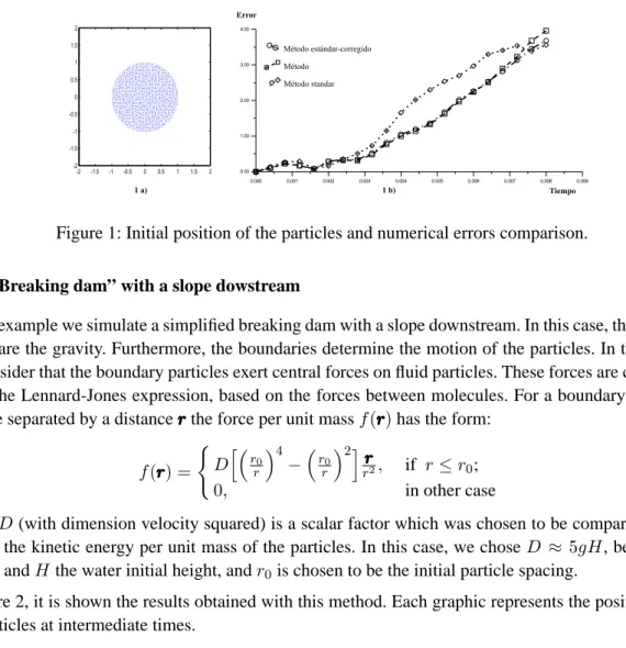
In figure 1 we show the results obtained using the standard SPH, the corrected SPH and the standard-corrected SPH. The parameters we use are:γ = 7,k = 285,714M N/m2 andρo = 1000kg/m3. In figure (1a) it can be observed the initial particle configuration. In all cases, we use1308 unstructured particles. In figure (1b) we compare the value of the productab. It could be equals1. The corrected SPH method and the standard-corrected method have a similar behaviour and the errors obtained are lower that those obtained with the standard SPH method.
Figure 1: Initial position of the particles and numerical errors comparison.
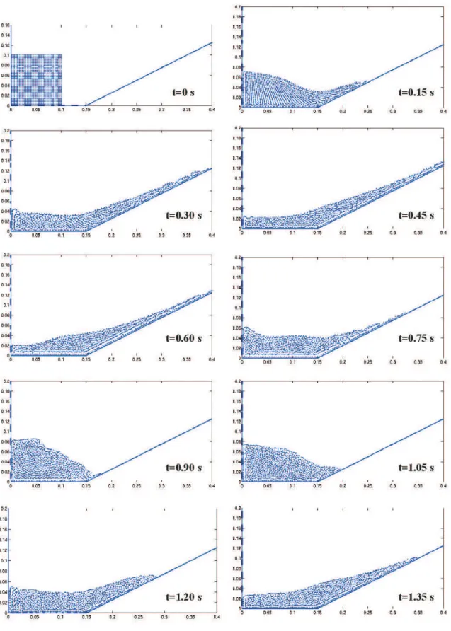
7.2 “Breaking dam” with a slope dowstream
In this example we simulate a simplified breaking dam with a slope downstream. In this case, the external forces are the gravity. Furthermore, the boundaries determine the motion of the particles. In this paper, we consider that the boundary particles exert central forces on fluid particles. These forces are calculated using the Lennard-Jones expression, based on the forces between molecules. For a boundary and fluid particle separated by a distancerrrrrrrrrrrrrrthe force per unit massf(rrrrrrrrrrrrrr)has the form:
f(rrrrrrrrrrrrrr) = (
D
h³ r0
r ´4
−
³ r0
r ´2i
rrrrrrrrrrrrrr
r2, if r≤r0;
0, in other case
(40)
whereD(with dimension velocity squared) is a scalar factor which was chosen to be comparable to or exceed the kinetic energy per unit mass of the particles. In this case, we choseD ≈ 5gH, beinggthe gravity andHthe water initial height, andr0is chosen to be the initial particle spacing.
In figure 2, it is shown the results obtained with this method. Each graphic represents the position of all the particles at intermediate times.
8 Conclusions
In this paper, the SPH method applied to free surface problems have been studied. Three different formu-lations have been analyzed: the standard SPH method, the corrected SPH method and standard-corrected SPH method. In both cases, first we have approached the equations that represents the physical problem we try to solve, then we have selected the points or particles where we want to calculate the solution and, finally, we have approximated the differential equation in spacial and in time dimensions and we have replaced it by an algebraic equation. Furthermore, we have center our attention in the approach of the corrections applied to preserve linear and angular momentums.
The standard-corrected SPH method allows to analyze the influence of the corrections that have been introduced in the formulation and the importance of the viscosity terms. The conclusion is that the cor-rection factors improve the accuracy of the results more than the use of a natural viscosity.
WCCM V, July 7–12, 2002, Vienna, Austria
Figure 2: Time evolution of fluid particles in a “breaking dam” problem with a slope downstream
9 Acknowledgements
This work has been partially supported by the SGPICT of the “Ministerio de Ciencia y Tecnolog´ıa” of the Spanish Government, cofinanced by research fellowships of the R&D Secretary of “Xunta de Galicia” and the “Universidade de A Coru˜na”.
References
[1] J.J. Monaghan Simulating Free Surface Flows with SPH, Annu. Rev. Astron. Astrophys., 30, 543-574; 1992
[2] T. Belytschko, Y. Krongauz, D. Organ, M. Fleming and P. Krysl Meshless methods: An overview and
recent developments Comput. Methods in Appl. Mech. and Engrg., 139,3-49; 1996
[3] J. Bonet, T.S.L. Lok Variational and momentum preseving aspects of Smooth Particle
Hydrodynam-ics formulations Comput. Methods in Appl. Mech. and Engrg., 180,97-115; 1998
[4] S. Fern´andez-M´endez Mesh-Free Methods and Finite Elements: Friend or Foe? Doctoral Thesis. Barcelona ; September 2001
[5] M.E. Gurtin An Introduction to Continuum Mechanics Mathematics in Science and Engineering, 158, Academic Press; 1981
[6] F.M. White Mec´anica de fluidos McGraw-Hill; 1983
[7] P.W. Randles, L.D. Libersky SPH: Some recent improvements and applications Comput. Methods in Appl. Mech. and Engrg., 139,375-408; 1996
[8] O.C. Zienkiewicz and K. Morgan Finite Elements and Approximation John Wiley & Sons, Inc; 1983
[9] S. Kulasegaram Development of Particle Based Meshless Method with Applications in Metal
Form-ing Simulations Doctoral Thesis. University of Wales Swansea; March 1999
[10] W. K. Liu, S. Jun & Y.F. Zhang Reproducing Kernel Particle Methods Int. J. Num. Meth. Engrg., 20; 1995
[11] T. Belytschko, Y. Krongauz, J. Dolbow, and C. Gerlach On the Completeness of Meshfree Particle
Methods Int. J. Num. Meth. Engrg., 43,785-819; 1998
[12] G. Mosqueira, I. Colominas, J. Bonet, F. Navarrina, M. Casteleiro Development of integration
schemes for meshless numerical approaches based on the SPH method. ECCOMAS CFD 2001,
Swansea, 4-7 September 2001.
[13] L. Cueto-Felgueroso, G. Mosqueira, I. Colominas, F. Navarrina, M. Casteleiro An´alisis de
for-mulaciones num´ericas SPH para la resoluci´on de problemas de flujo en superficie libre M´etodos
Num´ericos en Ingenier´ıa V, Madrid, 4-7 June 2002.