Effect of parameters on Geoa/Geob/1 Queues: theoretical analysis and simulation results

(1)

http://www.scirp.org/journal/am ISSN Online: 2152-7393

ISSN Print: 2152-7385

DOI: 10.4236/am.2018.92011 Feb. 28, 2018 153 Applied Mathematics

Effect of Parameters on Geo

a

/Geo

b

/1 Queues:

Theoretical Analysis and Simulation Results

A. Lorente

1*

, M. S. Sánchez

2

1_{Departamento de Matemáticas y Computación, Universidad de Burgos, Escuela Politécnica Superior, Avda. Cantabria s/n, 09006}

Burgos, Spain

2_{Departamento de Matemáticas y Computación, Universidad de Burgos, Facultad de Ciencias, Pza. Misael Bañuelos s/n, 09001}

Burgos, Spain

Abstract

This paper analyzes a discrete-time Geoa_/Geob_{/1 queuing system with batch} arrivals of fixed size a, and batch services of fixed size b. Both arrivals and ser-vices occur randomly following a geometric distribution. The steady-state queue length distribution is obtained as the solution of a system of difference equations. Necessary and sufficient conditions are given for the system to be stationary. Besides, the uniqueness of the root of the characteristic polynomial in the interval (0, 1) is proven which is the only root needed for the computa-tion of the theoretical solucomputa-tion with the proposed procedure. The theoretical results are compared with the ones observed in some simulations of the queuing system under different sets of parameters. The agreement of the re-sults encourages the use of simulation for more complex systems. Finally, we explore the effect of parameters on the mean length of the queue as well as on the mean waiting time.

Keywords

Discrete-Time Queuing System, Batch Arrivals, Batch Services, Stationary Systems

1. Introduction

Queuing systems are being studied from the beginning of the XX century, trying to model fluctuations arising in a queue, such as number of clients, waiting time, service time, etc. In fact, its origin can be found in the study of congestion prob-lems on telephone networks. The first work on these probprob-lems was published in 1909 by Agner Krarup Erlang [1] who demonstrated that telephone calls were

How to cite this paper: Lorente, A. and Sánchez, M.S. (2018) Effect of Parameters on Geoa_/Geob_{/1 Queues: Theoretical}

Anal-ysis and Simulation Results. Applied Ma-thematics, 9, 153-170. This work is licensed under the Creative Commons Attribution International License (CC BY 4.0).

http://creativecommons.org/licenses/by/4.0/

(2)

DOI: 10.4236/am.2018.92011 154 Applied Mathematics

well modeled by a Poisson distribution.

Besides the queues in the telephone exchanges that were the origin of the theory of queues, nowadays, batch queues are common in transports, distribution and telecommunications. Consequently, the words “customers” or “clients” are used in general terms, whether it is about people or, say, printer jobs waiting their turn. Chaudhry and Templeton [2] offer a complete analysis of queuing systems.

In particular, models in discrete-time have received much attention in the last years, mostly focusing on the calculus of the length queue distribution and wait-ing time. In pursuwait-ing these goals, different approaches are used and with differ-ent models that arise when considering varying characteristics such as the ser-vice policy, or distribution of arrivals or of inter-arrivals time.

The present paper focuses on discrete time queuing systems for batch arrivals and services, both following a geometric distribution and both with fixed size, though different. Following the notation introduced by Kendall [3], this is de-noted as Geoa_/Geob_/1.

A general discrete time GIX_/GY_{/1 model was studied by Alfa and He}_[4]_{by the} Markov chain associated to the number of customers in the queue. Chaudhry and Gupta [5] compute the length queue distribution and the waiting time through the PGF (Probability Generating Function) of the distributions involved for the GIX_{/Geo/1 model, and more recently,}_[6]_{, they focus on the waiting time} for the GIX_{/G/1 model. In}_[7]_{, Chaudhry and Kim present a multi-server model} with deterministic service times.

In [8], Borkakaty et al. focus on the busy period of the system GIa_/Gb_{/1, with} fixed sizes for arrival and service batches by lattice path approach. The method is first applied for models in discrete time, handling then the model in continuous time as the limiting case.

For arrivals of variable size following a Poisson distribution, Claeys et al. [9]

analyze the model MX_/GIl,c_{/1, where the server remains idle until there is at least}

l customers waiting and can serve at most c customers simultaneously. With geometric distribution for arrivals and services, in [10], they present the model GeoX_/Geoc_{/1 under two different policies: in the first, the server starts a new} ser-vice although the number of clients does not reach c; in the second, the server waits until the number of clients reaches c.

A related model, the GI/Geo/1 queue under N-policy, is analyzed by Lim et al.

[11]. In this model, customers arrive and are served one by one, but the server waits until the number of customers reaches N before starting services.

Bruneel et al.[12] examine the model with fixed service capacity, while in [13]

they consider systems with variable service capacity. Focusing in the interval between arrivals (keeping it constant) and constant time of service, Zhao and Campbell [14] use the roots, both inside and outside the unit circle, of the de-nominator of the generating function for the system DX_/Dm_{/1. Related to this} methodology, Janssen and Leeuwaarden [15] discuss about the method of find-ing the roots of

( )

s

A z −z (where A(z) is the PGF of the number of arriving

(3)

interpreta-DOI: 10.4236/am.2018.92011 155 Applied Mathematics

tion of the roots and to find them numerically. They present a solution for the stationary queue length distribution that does not depend on roots.

On the other hand, Yao et al.[16] consider computer simulation for discrete models as a method to avoid the difficulties of theoretical analysis.

The present paper shows how the specific characteristics of the model being studied make it possible to obtain the theoretical solutions without the need of finding all the roots of

( )

s

A z −z . In particular, we prove the existence of a

unique root of the characteristic polynomial in (0, 1), which suffices to obtain the solution, provided the system is stationary. Conditions for the system to be stationary are also given.

2. Analytic Solution

2.1. Model Description

The model under study is a discrete-time model denoted as Geoa_/Geob_/1: cus-tomers arrive in batches of fixed size a, and they are served in batches of fixed size b. If there is not at least b customers at the end of a service, the server does not start a new service until the number of waiting customers reaches b.

It is assumed that arrivals are independent, service times are independent, and services are independent of arrivals unless the number of waiting customers were less than b. Batch sizes a and b are supposed to be relative prime integers; otherwise, we would take their greatest common divisor as unit.

At each time slot, an arrival of a customers can happen with probability α, or not, with probability 1 − α. Furthermore, if there is a service running, it can finish with probability β, or not, with probability 1 − β. Besides, inter-arrival times are geometrically distributed with parameter α, and service times are geo-metrically distributed with parameter β. Then, traffic density is ρ=aα

( )

bβ .

Therefore, if there are n customers in the system, Equations (1) to (4) describe the different probabilities.

(

|

)

(

no arrival and no exit |

_{) ( )( )}

1 if

If the system reaches an equilibrium, and qn denotes the probability of “n

customers in the system”, then the following Equation (5) holds,

(4)

where all qm with m < 0 are 0.

Note that, according to Equations (1)-(4), the probabilities of exit or no exit are different depending on whether n is greater than b or not. Consequently, all equations with any subscript less than b are particular equations.

Since the lowest subscript in Equation (5) is n−a, then there are a b+

par-Remember that a and b are supposed to be relative prime integers. In any case, if a=b, the problem would reduce to a= =b 1, since each block can be treated

as a unit.

The general equation for n≥ +a b in Equation (12) is obtained by replacing

Equations (1)-(4) into Equation (5).

(

1

)(

1

)

(

1

)

(

1

)

The steady-state distribution, if it exists, must be a particular solution of Equ-ation (13). The general solution of EquEqu-ation (13) is

(

)

n

n k k

k

q =

∑

a x n≥ +a b

(15)

where

x

k are the roots of the characteristic polynomial in Equation (14).

Then, with the aim of studying the roots of Equation (14), we distinguish two cases:

Case

a b

<

:

If a<b, exponents in Equation (14) are already in ascending order. As a

(5)

By differentiating again the polynomial S(x) in Equation (18) is

( )

(

)

(

)(

)

(

)(

)

Like in the previous case, the second factor in Equation (19) is an increasing polynomial in the interval

(

0,∞

)

and negative at 0. Then S x′

( )

has a unique root in

(

0,∞

)

. This implies that S(x) has at most two roots in

(

0,∞

)

, and so

has P x′

( )

.

As S x′

( )

must be negative until its unique root in

(

0,∞

)

and positive after

the root, S(x) is at first decreasing, it reaches a relative minimum and turns to be an increasing function. Because S

( )

0 >0, either S(x) remains above the

hori-zontal axis in

(

0,∞

)

(maybe reaching it at the relative minimum), or S(x)

(6)

cannot construct any particular solution as defined in Equation (15), which should generate a probability distribution.

On the other hand, if aα<bβ , the root of P(x) in

( )

0,1 is unique, let x0

is a convergent series with positive terms. We can choose u>0 such that

Inserting Equation (23) into Equation (21), the probability of n customers in the system, qn, for n≥ +a b, is written as

depending on the first a b+ probabilities of the succession. We determine

these initial probabilities by replacing qn

(

n≥ +a b

)

in the a b+ particular

equations and solving the resulting linear system.

This provides the distribution of the total number of customers. Equation (25) gives the rule to obtain the number of customers waiting before service

(

customers waiting

)

if

Also from these equations, the average number of customers in the system is calculated by summing up the series in the following Equation (26)

1 1

and the average number of customers waiting is computed as:

(7)

3. Numerical Results and Discussion

3.1. Theoretical Probabilities versus Relative Frequencies

The equations in the previous section can be easily programmed so they provide a straightforward procedure to compute the probabilities. To illustrate the pro-cedure as well as comparing the probabilities against relative frequencies com-puted with simulated results (for the cases where the probabilities were difficult to compute), we simulated the system for some given values and for around 10,000 cycles. For the sake of simplicity, the case studies we chose were with small numbers for a and b.

near system obtained by substituting and rearranging Equations (6)-(8), and (12) (the details can be found in [17]), namely

the system, with different traffic density ρ obtained by varying the probability of incoming customers α. The probabilities have been computed for the total number of customers (first three columns) and also for the number of customers that are waiting (last three columns). The last row of Table 1 shows the corres-ponding expectation.

(8)

DOI: 10.4236/am.2018.92011 160 Applied Mathematics Table 1. Theoretical probabilities and expectations for the system with a = 2, b = 3, β = 0.5, and different traffic density ρ.

Total number

Expectation: 2.4319 6.4891 Expectation: 1.2473 4.1065

(9)

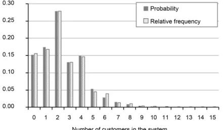
DOI: 10.4236/am.2018.92011 161 Applied Mathematics Figure 1. Results for the system with a = 2, b = 3, β = 0.5, α = 0.3 (ρ = 0.4).

Figure 2. Results for the system for a = 2, b = 3, β = 0.5, α = 0.6 (ρ = 0.8).

probabilities greater than 0.13 for less than 5 customers; while the remaining ones are very small, graphically inappreciable in Figure 1 from around 11 cus-tomers in the system, and smaller than 10−4_{from 17 customers (}_{Table 1}_).

The magnitude of q2 stands out clearly that reflects the fact that there must be at least 3 customers for the system to start, but they arrive two by two with less probability. Accordingly, the expectation is near 2 customers (2.4319 as can be seen in the last row of Table 1) in the system.

This same reason explains the behavior of the probabilities for the number of customers that are waiting their turn, fourth column in Table 1, not only the fact that the largest probability is indeed for 2 customers but that the cumulative probability of having up to 2 customers waiting is in fact 0.9378, almost the whole distribution.

(10)

ob-DOI: 10.4236/am.2018.92011 162 Applied Mathematics

viously less than their counterparts, and the expectation drops to 1.2473 customers. The difference between the first five probabilities and the remaining ones is less pronounced in the second system, with ρ = 0.8, as we can see in both Figure 2 and the third column of Table 1 and also for the probabilities of n customers waiting to go to the server, last column in Table 1.

In Figure 2, again, there is not difference between the probabilities computed with Equation (24) and the relative frequencies obtained when simulating the system (except may be for 6 customers in the system), the probability reaches its maximum for 4 customers (0.1428 in Table 1) but then, contrary to the situation in Figure 1, the probabilities softly decrease and remain larger than 8 × 10−4_for up to 30 customers. The expectation increases accordingly up to near 6.5 cus-tomers in the system, on average, 4 of them waiting.

Like in the previous case, when looking at the probability of having n custom-ers waiting for their turn, the largest probability is for 2 customcustom-ers waiting, and again the largest probabilities are indeed for 0, 1 or 2 customers waiting but now the cumulative probability is much smaller, 0.5514, and slowly decreases from 3 customers waiting their turn.

In this case, larger traffic density due to the larger probability of arrival causes larger probabilities for more customers in the system, and thus for the ones waiting because the probability of service is the same.

For illustrative purposes, Table 2 contains probabilities and relative frequen-cies computed also with ten thousand cycles when a > b, in this case, obtained for a = 5, b = 3, and probabilities α = 0.2, β = 0.4 (thus, maintaining high traffic density ρ = 0.83). The range of values shown now for the number of customers is necessarily larger than in Table 1 because the root of the characteristic poly-nomial is 0.9392 implying a very slow decreasing of the probabilities when in-creasing the number of customers for

n

≥ = +

8 a

b

, see Equation (24).

As in the previous case, the results for the number of total customers in the system are similar to each other, although in this case, shorter simulation times showed rather high differences between the theoretical probabilities and the ob-served frequencies.

The largest values are in the first three rows, up to 2 customers in the system, especially for exactly 2 customers. This is due to the needed 3 = b customers to start the service. Then, from 3 to 7 = a + b −1 customers, both the probabilities and observed frequencies increase and, at that point, they start to slowly de-crease from 8 customers in the system, although the high traffic density diffuses the differences among these three block of probabilities (or frequencies). The slow decrease is apparent in the fact that there is still 0.8 in a thousand rate of having 70 customers in the system, with almost 16 customers on average, 15.72 according to Table 2.

3.2. Effect of the Parameters on the Queue Length and Waiting

Time

(11)

DOI: 10.4236/am.2018.92011 163 Applied Mathematics Table 2. Relative frequencies observed in a simulation of 10,000 cycles and theoretical probabilities computed for a = 5, b = 3, α = 0.2, β = 0.4.

Total number

of customers frequency Relative Probability Total number of customers frequency Relative Probability

(12)

the length of the queue, in the two possible situations a < b and b < a, we main-tain the size of the blocks, both entering and exiting the system (the same as in section 3.1), and modify the rate service from high (β = 0.2), medium (β = 0.5), to low (β = 0.7). Systematic simulations were conducted by varying the arrival rate α with the purpose of obtaining traffic density ρ from 0.1 to 0.9.

In all cases, Equations (27) and (28) are used to compute the average number of customers in the system and the average number of customers waiting for service. The average waiting time is obtained from simulations. From it, we also computed the percentage of this waiting time due to the insufficient number of customers in the system, i.e. the time spent waiting for the system to reach the minimum b customers to start a service.

The first situation corresponds to the first system studied in Section 3.1, and thus the simulations and computation are made by keeping a = 2 and b = 3. The resulting waiting time is depicted in Figure 3 as a function of the traffic density, and for the three values of β taken into account in order to cover slow, medium and fast services, namely β = 0.7, β = 0.5 and β = 0.2, respectively.

It is observed that, for all values of β, the average waiting time is rather high for low traffic density, probably because customers must wait until the number reaches the minimum b. It decreases slowly until medium traffic density and then grows up again for high traffic density due to congestion.

As expected, irrespective of ρ, the time spent waiting decreases with β but not in the same way. The differences among mean times for each ρ_{are larger when}

comparing the slow service (open circles) to the medium one (crosses), with smaller differences between the later and the fast one (filled circles). These dis-tances are remarkably different above all for extreme traffic densities, notice the huge increase in the mean for ρ = 0.9 when β = 0.7 as compared to the medium or the fast one.

This behavior is related to the one depicted in Figure 4, the percentage of the

(13)

DOI: 10.4236/am.2018.92011 165 Applied Mathematics Figure 4. Percentage of waiting time with the server free vs. traffic densi-ty for a = 2, b = 3, and different β.

waiting time that is due to inactivity of the server because there are not enough customers waiting for service, i.e., the server is free but the customers are wait-ing. At low traffic density, irrespective of the probability of the service, most of the waiting time is due to the insufficient number of customers. For instance, when ρ = 0.1, more than 90% of the total waiting time is spent with the server idle (thus, the increasing mean value of the total waiting time already observed in Figure 3). As expected, the values coincide again, practically null in this case, for ρ = 0.9, where the traffic is so high that more than 90% of the time that the customers spent waiting is because the server is busy (only less than 5% of the waiting time is due to insufficient customers).

Between these two extreme values, Figure 4 shows a decreasing behavior of the percentage of the time waiting for the minimum number of customers needed to start the service, a decreasing which is almost linear for the fastest ser-vice among the cases shown. Globally, for a given traffic density, the faster the service is, the larger the percentage of the time spent waiting that is due to the fact that there are not enough customers.

In relation to the number of customers in the system, Figure 5 shows the av-erage values for both the total number of customers (black lines) and the num-ber of them waiting for service (in red lines). As expected, in both cases, the mean values are ordered from smallest to largest according to the speed of the service, i.e., the largest mean values are for the slow service (open circles or squares for the total number of customers or for those waiting, respectively), then the ones corresponding to the medium service rate (crosses in Figure 5), and the smallest mean values are for the fast service (filled circles or squares).

(14)

DOI: 10.4236/am.2018.92011 166 Applied Mathematics Figure 5. Average number of both total customers (dark lines) and custom-ers waiting for service (red lines) vs. traffic density for a = 2, b = 3, and dif-ferent rate services (β = 0.7 for slow, β = 0.5 for medium and β = 0.2 for fast services).

0.4. From then, the mean values continue their increase with ρ, but the differ-ences due to β become apparent, more importantly for largest traffic densities and also with more dispersion, that is, larger differences among the averages correspond to larger values of ρ, though this dispersion is the same for the total number of customers or when we look only to the customers that are waiting.

Similar conclusions can be drawn with systems with a = 5 and b = 3 (then a > b, as opposed to the preceding case). Figure 6 shows the effect of traffic density on the mean waiting time computed with the simulations conducted, as before, modifying the rate service from high (β = 0.2), medium (β = 0.5), to low (β = 0.7) and varying the arrival rate α with the purpose of obtaining traffic density ρ from 0.1 to 0.9.

The pattern in Figure 6 is the same as the one observed in Figure 3, at first decreasing with the increase of ρ up to approximately 0.5 and then a faster in-crease of the waiting time when ρ continues to increase. However, in the present case the mean waiting time is comparatively larger in all cases, especially in the slow service, open circles in Figure 6.

It might seem obvious because customers arrive in groups of a = 5 instead of a = 2 but, in fact, it was not so predictable because the rate of arrival is also varying so that the product remains constant; in other words, there are more clients ar-riving but they do so more spaced in time to maintain traffic density. When comparing to Figure 7 that shows the percentage of the time spent waiting be-cause there are not enough customers to start a service, the reason becomes clearer, they are waiting for attention, because for every five arriving, at most three receive service thus there can be up to four customers waiting and still one when the next service starts. This percentage is now smaller, although, as in

(15)

DOI: 10.4236/am.2018.92011 167 Applied Mathematics Figure 6. Mean waiting time vs. traffic density for a = 5, b = 3, and dif-ferent β.

Figure 7. Percentage of the total waiting time with the server free vs. traf-fic density for a = 5, b = 3, and varying β.

traffic density increases (up to a point).

Comparing to the case a < b, the decreasing pattern for all values of β is now less linear than it appeared to be in Figure 4 and also the differences among the percentages for the three service rates are smaller than the ones observed in Fig-ure 4. This reflects the fact that with a > b the server is less frequently free.

Figure 8 shows the average number of total customers (in black) and the av-erage of the number of customers waiting for service (in red lighter lines), among those in the system. The global increasing pattern of the mean values when increasing the traffic density is the same as the one observed for a < b in

Figure 5, but now the average number of customers, both total or waiting, is al-ways higher than it was for the analogous case.

(16)

DOI: 10.4236/am.2018.92011 168 Applied Mathematics Figure 8. Average number of total customers in the system (black lines) and average number of waiting customers (red lines) vs. traffic density for a = 5, b = 3. Different service rate: slow for β = 0.7, medium β = 0.5, and fast for β = 0.2.

and, consequently, there are more customers (both total customers and the number of them that are waiting). It is remarkable the sharp increase of the mean number of customers when passing from traffic density 0.8 to 0.9.

4. Conclusions

In this paper, we present a discrete-time queuing system where both arrivals and services occur in batches of fixed size, a for arrivals and b for services, following geometric distributions with probabilities α and β, respectively. In this situation, analytical solutions are obtained by explicitly establishing the steady-state equa-tions, and proving that that the system is stationary if and only if aα<bβ .

The specific features of the system allow us avoiding the search of all roots of

( )

s

A z −z when computing probabilities, since it suffices to take into account

the unique real root of the characteristic polynomial in (0, 1), if the stationary requirements hold.

Simulations of the system conducted under different sets of parameters show the similarity between the theoretical probabilities and the relative frequencies obtained in the numerical results. This provides a viable alternative to avoid solving the whole set of equations for each particular case, and then compute the remaining probabilities.

(17)

Acknowledgements

Special thanks are due to Dr. M.ª Cruz Valsero, former professor at the Univer-sity of Valladolid (Spain) for her encouragement, and useful discussions.

References

[1] Erlang, A.K. (1909) The Theory of Probabilities and Telephone Conversations. Nyt Tidsskrift for Matematik B, 20, 33.

[2] Chaudhry, M.L. and Templeton, J.G.C. (1983) A First Course in Bulk Queues. Wiley, New York.

[3] Kendall, D.G. (1953) Stochastic Processes Occurring in the Theory of Queues and Their Analysis by the Method of the Imbedded Markov Chain. The Annals of Mathematical Statistics, 24, 338-354. https://doi.org/10.1214/aoms/1177728975 [4] Alfa, A.S. and He, Q.M. (2008) Algorithmic Analysis of the Discrete Time GIX_/_GY_/1

Queueing System. Performance Evaluation, 65, 623-640. https://doi.org/10.1016/j.peva.2008.02.001

[5] Chaudhry, M.L. and Gupta, U.C. (1997) Queue-Length and Waiting-Time Distri-butions of Discrete-Time GIX_{/Geom/1 Queueing Systems with Early and Late}

Arri-vals. Queueing Systems, 25, 307-324. https://doi.org/10.1023/A:1019144116136 [6] Chaudhry, M.L. and Gupta, U.C. (2001) Computing Waiting-Time Probabilities in

the Discrete-Time Queue: GIX_/G/1._{Performance Evaluation}_{, 43, 123-131.}

https://doi.org/10.1016/S0166-5316(00)00038-9

[7] Chaudhry, M.L. and Kim, N.K. (2003) A Complete and Simple Solution for a Dis-crete-Time Multi-Server Queue with Bulk Arrivals and Deterministic Service Times. Operations Research Letters, 31, 101-107.

https://doi.org/10.1016/S0167-6377(02)00214-6

[8] Borkakaty, B., Agarwal, M. and Sen, K. (2010) Lattice Path Approach for Busy Pe-riod Density of GIa_/_Gb_{/1 Queues Using}_C

2 Coxian Distributions. Applied

Mathe-matical Modelling, 34, 1597-1614. https://doi.org/10.1016/j.apm.2009.09.005 [9] Claeys, D., Walraevens, J., Laevens, K. and Bruneel, H. (2007) A Discrete-Time

Queuing Model with a Batch Server Operating under the Minimum Batch Size Rule. NEW2AN2007: Next Generation Teletraffic and Wired/Wireless Advanced Net-working, 4712, 248-259. https://doi.org/10.1007/978-3-540-74833-5_21

[10] Claeys, D., Walraevens, J., Laevens, K. and Bruneel, H. (2010) Delay Analysis of Two Batch-Service Queueing Models with Batch Arrivals: GeoX_/_Geoc_{/1. 4}_OR_{, 8,}

255-269. https://doi.org/10.1007/s10288-009-0111-2

[11] Lim, D.E., Lee, D.H., Yang, W.S. and Chae, K.C. (2013) Analysis of the GI/Geo/1 Queue with N-Policy. Applied Mathematical Modelling, 37, 4643-4652.

https://doi.org/10.1016/j.apm.2012.09.037

[12] Bruneel, H., Rogiest, W., Walraevens, J. and Wittevrongel, S. (2015) Analysis of a Discrete-Time Queue with General Independent Arrivals, General Service Demands and Fixed Service Capacity. Mathematical Methods of Operations Research, 82, 285-315. https://doi.org/10.1007/s00186-015-0515-z

[13] Bruneel, H., Wittevrongel, S., Claeys, D. and Walraevens, J. (2016) Discrete-Time Queues with Variable Service Capacity: A Basic Model and Its Analysis. Annals of Operations Research, 239, 359-380. https://doi.org/10.1007/s10479-013-1428-y [14] Zhao, Y.Q. and Campbell, L.L. (1996) Equilibrium Probability Calculations for a

(18)

https://doi.org/10.1007/BF01159401

[15] Janssen, A.J.E.M. and van Leeuwaarden, J.S.H. (2005) Analytic Computation Schemes for the Discrete-Time Bulk Service Queue. Queueing Systems, 50, 141-163. https://doi.org/10.1007/s11134-005-0402-z

[16] Yao, M.H., Chen, X.J. and Zuo, L.C. (2014) Customer Arrival Event Processing on Computer Simulation for Discrete Event System. Applied Mechanics and Materials, 513-517, 2133-2136.

https://doi.org/10.4028/www.scientific.net/AMM.513-517.2133