Is a “Soft” monetary authority appropriate?
22
0
0
Texto completo
(2) ENSAYOS DE POLÍTICA ECONÓMICA – AÑO 2017 ISSN 2313-979X - Año XI Vol. II Nro. 5. Is a "Soft" Monetary Authority Appropriate? Carlos Esteban Posada5 y Alfredo Villca6 Resumen Teniendo como marco de referencia la “estrategia de inflación objetivo” es usual discutir lo que es más conveniente para una sociedad en cuanto al grado de “dureza” o “agresividad” de una autoridad monetaria para defender su meta de inflación, y la credibilidad de que esta goza entre los agentes económicos. En este documento utilizamos un modelo de equilibrio general dinámico estocástico (DSGE, por sus siglas en inglés) neo-keynesiano tanto con expectativas racionales como adaptativas para analizar esta cuestión y, además, cuantificamos los efectos de estos dos tipos de autoridades sobre el bienestar social utilizando una función de utilidad convencional. Nuestros resultados sugieren que el problema que se puede derivar de una autoridad “blanda” es arriesgar la pérdida de credibilidad en su (supuesto) empeño para alcanzar una determinada meta de inflación. Además, presentamos y utilizamos una solución del modelo lo suficientemente simple como para permitir que sus simulaciones sean implementadas en una hoja de cálculo.. Códigos JEL: C63, C68, E31, E32, E37, E58 Palabras claves: Objetivos de Inflación, Autoridad Monetaria, Modelos de Equilibro General Estocástico Dinámico, Regla de Taylor, Credibilidad.. Abstract. Taking the "objective inflation strategy" as a frame of reference, it is usual to discuss what is most convenient for a society in terms of the degree of "hardness" or "aggressiveness" of a monetary authority to defend its inflation target, and the credibility it has among the economic agents. In this document we use a NeoKeynesian Stochastic Dynamic General Equilibrium (DSGE) model both with rational and adaptive expectations to analyze this question and we also quantify the effects of these two types of authorities on social welfare using an utility function. Our results suggest that the problem that can be derived from a "soft" authority is to risk the loss of credibility in its (supposed) effort to reach a certain inflation target.. 5. Professor, Economics Department, Universidad EAFIT, Colombia. E-mail address: [email protected] 6. PhD degree student, Economics Department, Universidad EAFIT, Colombia. E-mail address: [email protected]. We thank the anonymous referees for contributing to this paper better. 57.
(3) In addition, we present and use a solution of our model simple enough to allow other simulations related to this class of models to be implemented in a spreadsheet.. JEL Codes: C63, C68, E31, E32, E37, E58 Key Words: Inflation Target, Monetary Authority, Dynamic Stochastic General Equilibrium Models, Taylor Rule, Credibility.. I. Introduction Monetary authorities often have an “Inflation Targeting” strategy, conditioning monetary policy, at least partially, to these one. This applies to many developed economies but also to several emerging economies. For example, the United Kingdom, Canada, New Zealand, Australia, Brazil and Chile adopted it in the 90s, and Turkey, Norway, Iceland, Romania, South Africa, Mexico, Colombia and Peru adopted it in the 2000s. Argentina, through the Central Bank, in 2016 has mentioned adopting the inflation target scheme. Figure 3 (Appendix B) shows the behavior of the 12-month inflation rate for emerging countries that apply the inflation-target scheme. It can be observed that during 2005-2016 the inflation rate was oscillating around the target, which means that the monetary policy was focused on fulfilling its objective. The most common strategy in this regard is to establish a policy of setting the short-term interest rate that leads to the achievement of the goal, without renouncing the achievement of other objectives, such as keeping closed the gap between the observed gross domestic product and the potential GDP. On the other hand, unforeseen variations (shocks) in the inflation rate are also frequent. These disturbances can be classified into two types according to their origin: aggregate supply and aggregate demand 7. Faced with such variations, the monetary authority can respond in a “hard” way (with measures that could be deemed “Draconian”, closing the inflation gap as soon as possible), or in a “soft” way, that is, with the slowness supposedly required to cause the least collateral damage possible but prolonging, perhaps for too long, an excessive inflation. Macroeconomic literature, under the neo-Keynesian approach, has studied the welfare effects of anticipated and unanticipated shocks (Davis, 2007, Fujiwara, Hirose, and Shintani, 2008 and Hans-Werner and Winkler, 2009) and explains that these are important factors of the aggregate fluctuations. However, the effects of the behavior of the monetary authority on welfare have not been explored yet. What is the best kind of monetary authority: hard o soft? To answer this question, we use two types of models; with the former, we assume that agents have rational 7. We suppose there is no interest rate shocks, i.e. that the monetary authority always has full control of the interest rate.. 58.
(4) ENSAYOS DE POLÍTICA ECONÓMICA – AÑO 2017 ISSN 2313-979X - Año XI Vol. II Nro. 5. expectations (Muth, 1961, Lucas, 1972 and 1973, and Sargent and Wallace, 1976), and with the latter we assume that they have adaptive expectations (Cagan, 1956, and Nerlove, 1958); the latter assumption allows a discussion on the credibility that the monetary authority enjoys to achieve and maintain (or recover) an inflation rate equal to the target. In both models the monetary authority has two objectives (inflation and output) and a single instrument (the interest rate), so given rise to two trade-offs (one of them intra-temporal; the other one inter-temporal) between inflation and product. Therefore, the policy maker need to face a painful choice. This is the subject of this paper, and it is organized as follows: section 2 explains the model; section 3 presents the simulation results, section 4 is an analysis of welfare effects, and section 5 concludes.. II. The Neo Keynesian Model. II.1. The model with Rational Expectations The first equation of the model, presented ahead, corresponds to the aggregate demand (or the neo Keynesian IS curve). It is derived from the Euler equation of the problem of inter-temporal utility maximization of consumers. Woodford (2003), Galí (2015), Menz and Vogel (2009), Walsh (2010) and Romer (2012), among others, present detailed treatments of this derivation. We start from a simple problem of consumer maximization raised in Wickens (2008, pp. 365), but explicitly including the price level.. ∞. 𝑈 = max 𝔼𝑡 ∑ 𝛽 𝑡 𝑢(𝑐𝑡 ) {𝑐𝑡 ,𝑎𝑡+1 }. 𝑡=0. Subject to the following restriction:. 𝑎𝑡+1 + 𝑝𝑡 𝑐𝑡 = 𝑥𝑡 + (1 + 𝑖𝑡 )𝑎𝑡. Where 𝑐𝑡 , 𝑎𝑡 , 𝑝𝑡 , 𝑥𝑡 and 𝑖𝑡 are consumption, financial asset, price level, exogenous labor income and nominal rate of return on financial assets (which are assumed to be risk-free assets). Taking into account the utility function with constant relative risk aversion; 𝑢(𝑐𝑡 ) = the Euler equation:. 𝑐𝑡1−𝜎 −1 1−𝜎 𝑐𝑡−𝜎. , and the first order conditions of the problem, we obtain. = 𝛽(1 + 𝑖𝑡 )𝔼𝑡 [. 𝑝𝑡 𝑐 −𝜎 ]. 𝑝𝑡+1 𝑡+1. Through log – linearization we can. immediately deduce the aggregate demand curve 8. The relationship obtained is the function describing the product gap, 𝑦𝑡 = ln 𝑌𝑡 − ln 𝑌𝑡∗ , in terms of its expected value,. In the process, we assume that the economy is closed, without government neither capital accumulation; therefore, product is equal to consumption. 8. 59.
(5) 𝔼𝑡 (𝑦𝑡+1 |Ω𝑡 ), and of the real interest rate, component:. 𝑖𝑡 − 𝔼𝑡 (𝜋𝑡+1 |Ω𝑡 ), plus a stochastic. 𝑦. 𝑦𝑡 = 𝔼𝑡 (𝑦𝑡+1 |Ω𝑡 ) − 𝛼[𝑖𝑡 − 𝔼𝑡 (𝜋𝑡+1 |Ω𝑡 )] + 𝜀𝑡. Where Ω𝑡 (∀ 𝑡 ∈ ℝ+ ). (1). is the set of available information about the variables, the. characteristics of its probabilistic distribution and the structure of the model, 𝛼 =. 1 𝜎. >. 0 is the inverse of the (constant) coefficient of risk aversion that captures the effect of the real interest rate on the output gap. Following again Wickens (2008, pp. 224), the problem facing the firm is to minimize the expected quadratic cost function given by the gap between the price, 𝑝, of the firm (the control’s variable) with respect to the optimal price, 𝑝𝑡∗ .. ∞ ∗ )2 min ∑ 𝜒 𝑠 𝔼𝑡 (𝑝𝑡 − 𝑝𝑡+𝑠 {𝑝𝑡 }. 𝑠=0. Where 𝜒 = 𝜃𝛽 is the stochastic discount factor given that 𝜃 is the probability of changing prices in the following period. The optimum price chosen by the firm is 𝑠 ∗ obtained from the first order condition, 𝑝̅𝑡 = (1 − 𝜒) ∑∞ 𝑠=0 𝜒 𝔼𝑡 (𝑝𝑡+1 ). To derive the Phillips curve we operated with this last expression taken into account that the price level of the economy is given by this law: 𝑃𝑡 = 𝜃𝑃𝑡−1 + (1 − 𝜃)𝑝̅𝑡 . The result is a functional relationship of the inflation gap (𝜋𝑡 = 𝜋𝑡𝑜𝑏𝑠 − 𝜋̅, where 𝜋̅ is the inflation target) in terms of its expected value and the output gap (see: Woodford, 2003, and Walsh, 2010). This equation is:. 𝜋𝑡 = 𝛽1 𝔼𝑡 (𝜋𝑡+1 |Ω𝑡 ) + 𝛽2 𝑦𝑡 + 𝜀𝑡𝜋. (2). Where 𝛽1 is the coefficient that captures the effect of the expected inflation rate on current inflation, and 𝛽2 is the effect of the output gap on the observed inflation ( 0 < 𝛽𝑗,(𝑗=1,2) < 1). The third equation describes the behavior of the monetary authority that abides to the Taylor’s rule (Taylor, 1993)9. The Taylor’s rule (including a purpose of smoothing the policy interest rate) is:. 𝑖𝑡 = 𝛾𝑖𝑡−1 + (1 − 𝛾)[𝜙1 𝔼𝑡 (𝑦𝑡+1 |Ω𝑡 ) + 𝜙2 𝔼𝑡 (𝜋𝑡+1 |Ω𝑡 )]. (3). See: Svensson (1997), Dennis (2004) and Walsh (2010) (among others) for theoretical justifications of the Taylor rule. 9. 60.
(6) ENSAYOS DE POLÍTICA ECONÓMICA – AÑO 2017 ISSN 2313-979X - Año XI Vol. II Nro. 5. Where 𝑖𝑡 it is the gap between the rate fixed by the monetary authority and the “neutral” rate (or sum of the equilibrium real interest rate and the inflation target; 𝑝𝑜𝑙. 𝑖𝑡 = 𝑖𝑡 − (𝑖𝑡𝑛 + 𝜋̅) ). The parameter 𝛾 refers to the procedure to smooth the movements of the interest rate (0 ≤ 𝛾 < 1). A monetary authority that we call “hard” is characterized by a relatively large parameter 𝜙2 . This authority complies with the Taylor’s principle (𝜙2 > 1 ), which means that if inflation rises then the policy rate must increase by a greater magnitude to hit the inflation target as quickly as possible. In addition, we call “soft” authority the one whose actions agree with those of a relatively small value of this parameter. 𝑗. In equations (1) and (2) the term 𝜀𝑡 is a stochastic variable having a first order auto-regressive structure:. 𝑗. 𝑗. 𝑗. 𝜀𝑡 = 𝜌𝑗 𝜀𝑡−1 + 𝜇𝑡 ;. 𝑗. 0<𝜌<1. (4). 𝑗. Where 𝜇𝑡. is a random shock (white noise) following a zero mean 𝔼(𝜇𝑡 ) = 0 𝑗. distribution with a constant variance 𝕍(𝜇𝑡 ) = 𝜎𝑗2 , for 𝑗 = 𝑦, 𝜋. Let 𝜃 = {𝛼, 𝛽1 , 𝛽2 , 𝛾, 𝜙1 , 𝜙2 , 𝜌𝑦 , 𝜌𝜋 } be the set of model parameters, and let 𝑋𝑡 = [𝑦𝑡 , 𝜋𝑡 , 𝑖𝑡 ]′ 𝑦. and 𝑍𝑡 = [𝜀𝑡 , 𝜀𝑡𝜋 , 0]′ be the transposed vectors of the endogenous and exogenous variables respectively. Hence, the model given by equations (1) – (3) can be represented in matrix form as follows:. Γ0 (𝜃)𝔼𝑡 (𝑋𝑡+1 |Ω𝑡 ) + Γ1 (𝜃)𝑋𝑡 + Γ2 (𝜃)𝑋𝑡−1 + Ψ0 (𝜃)𝑍𝑡 = 0. (5). Similarly, process (4) can be written in matrix form:. 𝑍𝑡 = Ψ1 (𝜃)𝑍𝑡−1 + 𝜉𝑡. The terms Γ𝑗 (𝜃),. for 𝑗 = 0,1,2, and Ψ𝑠 (𝜃), for 𝑠 = 0,1,. (6). are square matrices of. dimension 3 representing the model parameters. Furthermore, 𝜉𝑡 is a vector whose first two components are white noise and the third is zero. There are three (usual) methods for solving macroeconomic models with rational expectations, namely: indeterminate coefficients, recursive substitution and delay operators (see Blanchard and Kahn 1980, Christiano 2002, Sims 2002, and Lubik. 61.
(7) and Schorfheide 2003, among others). To solve equation (5) we use the first method for simplicity. For this, we conjecture a solution of the form 10:. 𝑋𝑡 = Φ(𝜃)𝑋𝑡−1 + Π(𝜃)𝑍𝑡. (7). To determinate the matrices of coefficients Φ(𝜃) and Π(𝜃) we advanced a period and apply conditioned rational expectations to the set of available information, whose result is combined with that obtained from advancing a period in equation (6), so much:. 𝔼𝑡 (𝑋𝑡+1 |Ω𝑡 ) = Φ(𝜃)𝑋𝑡 + Π(𝜃)Ψ1 (𝜃)𝑍𝑡. (8). Substituting (8) in (5) and rearranging we solve for the vector 𝑋𝑡 . This result is matched with (7). To solve the system obtaint a recursive strategy of approach convergent to the solution is adopted (fixed point method). To implement this procedure, we express the indexed system as follows:. Φ𝑖 (𝜃) = −[Γ0 (𝜃)Φ𝑖−1 (𝜃) + Γ1 (𝜃)]−1 Γ2 (𝜃) Π𝑖 (𝜃) = −[Γ0 (𝜃)Φ𝑖−1 (𝜃) + Γ1 (𝜃)]−1 [Γ0 (𝜃)Π𝑖−1 (𝜃)Ψ1 (𝜃) + Ψ0 (𝜃)]. (9) (10). The previous system can be written in compact form, for which let 𝐱 𝑖 = [Φ𝑖 (𝜃), Π𝑖 (𝜃)]′ be the transposed vector of unknowns variables and 𝐠(𝐱 𝑖−1 ) the set of the two expressions on the right side. In order to iterate, an arbitrary value (which implies that Φ0 (𝜃) and Π0 (𝜃) are given a priori), with which the recursive scheme 𝐠(𝐱 𝑖−1 ) starts , so that a sequence of vectors is generated until 𝐱 𝑖 and 𝐱 𝑖−1 , for some i, converge with each other, which implies that the Euclidean distance ‖ 𝐱 𝑖 − 𝐱 𝑖−1 ‖ between both approaches zero. Under this condition, the following optimization program is solved:. min‖ 𝐱 𝑖 − 𝐱 𝑖−1 ‖. For a certain i, we obtain the optimal vector 𝐱 ∗ given by the set [Φ∗ (𝜃), Π ∗ (𝜃)], which solves the previous optimization problem and in turn also solves system (9) and (10), and therefore model (7). Consequently, the impulse-response relationships are given by: 10. See Appendix A for the full solution.. 62.
(8) ENSAYOS DE POLÍTICA ECONÓMICA – AÑO 2017 ISSN 2313-979X - Año XI Vol. II Nro. 5. 𝑋𝑡 = Φ∗ (𝜃)𝑋𝑡−1 + Π ∗ (𝜃)𝑍𝑡. II.2. The model with adaptive expectations Now, we assume that agents form their expectations in an adaptive way, which means that they take into account only the information required to perform in a simple way a forecast that is subject to possible systematic errors, unlike the case of rational expectations that assumes that agents anticipate the future by making only random errors, using all available information (and the knowledge of the model that generates the observed data). For this reason, we preclude the discussion on credibility or disbelief upon the rational expectations case, whereas now is relevant. The structure of this model includes three equations similar to the previous model but, additionally, a rule for the process of formation of expectations is postulated. The first one specifies that the aggregate demand follows this law:. 𝑦. 𝑦𝑡 = 𝑦 ∗ − 𝛼(𝑖𝑡 − 𝜋𝑡𝑒 − 𝑟 𝑛 ) + 𝜀𝑡. (11). Where 𝑦 ∗ is the logarithm of the full-employment output (or long-run trend output), 𝜋𝑡𝑒 is the expected inflation, and 𝑟 𝑛 is the natural interest rate. On the other hand, observed inflation is related to the expected rate and the output gap; the later due to supply pressures associated to this gap. This hypothesis confirms the Phillips curve (similar to equation 2):. 𝜋𝑡 = 𝛽1 𝜋𝑡𝑒 + 𝛽2 (𝑦𝑡 − 𝑦 ∗ ) + 𝜀𝑡𝜋. (12). The third hypothesis is the Taylor rule:. 𝑖𝑡 = 𝛾𝑖𝑡−1 + (1 − 𝛾)[𝑟 𝑛 + 𝜋𝑡𝑒 + 𝜙1 (𝑦𝑡 − 𝑦 ∗ ) + 𝜙2 (𝜋𝑡 − 𝜋̅)]. (13). The remaining parameters and variables have the same characteristics and meaning as in the rational expectations model but (in addition) a rule is established for the inflation’s expectations, namely:. 𝜋𝑡𝑒 = 𝜆𝜋𝑡−1 + (1 − 𝜆)𝜋̅. (14) 63.
(9) Where 0 ≤ 𝜆 ≤ 1 is a parameter of partial adjustment of expectations. To understand better the expression (14) we can rewrite it as follow: 𝜋𝑡𝑒 = 𝜋̅ + 𝜆(𝜋𝑡−1 − 𝜋̅) which means that current expectations of future inflation reflect the target plus an error term given by 𝜆(𝜋𝑡−1 − 𝜋̅) related to the gap between the past inflation and the target. Equation (14) is also interpreted as a rule associate with relatively high or low values given to the weighting of the inflation target, that is, to the degree of credibility that the monetary authority has to adjust the observed inflation rate to the target in a relatively fast time in the event of occurrence of some mismatch in this respect. The perturbation terms in equations (11) – (12) follow a first order self-regressive structure similar to that assumed in the rational expectations model. Solving this type of models is simple. We substitute (13) in (11); it follows that:. 𝜋𝑡 = 𝛽1 𝜆𝜋𝑡−1 + 𝛽1 (1 − 𝜆)𝜋̅ + 𝛽2 𝑦𝑡 − 𝛽2 𝑦 ∗ + 𝜀𝑡𝜋. (15). On the other hand, we replace (13) in (11) and after a simplification, and applying again (14), we deduce the solution for 𝑦𝑡 :. 𝑦. 𝑦𝑡 = 𝑦 ∗ + 𝑎1 𝜋𝑡−1 + 𝑎2 𝑖𝑡−1 + 𝑎3 𝜋𝑡 + 𝑎4 + 𝑎5 + 𝑎6 𝜀𝑡. (16). Finally, we substitute (16) in (15) to obtain the solution of 𝜋𝑡 :. 𝑦. 𝜋𝑡 = 𝑏1 𝜋𝑡−1 + 𝑏2 𝑖𝑡−1 + 𝑏3 + 𝑏5 𝜀𝑡 + 𝑏6 𝜀𝑡𝜋. (17). Expressions (16) and (17) together with (13) allow solving the model, where:. 𝑎1 =. 𝑎4 =. 𝛼𝛾𝜆 ; 1 + 𝛼𝜙1 (1 − 𝛾). 𝑎2 = −. 𝑎3 = −. 𝛼𝛾(1 − 𝜆) + 𝛼𝜙2 (1 − 𝛾) 𝛼𝛾 𝜋̅ + 𝑟𝑛 ; 1 + 𝛼𝜙1 (1 − 𝛾) 1 + 𝛼𝜙1 (1 − 𝛾) 𝑏1 =. 𝛽1 𝜆 + 𝑎1 𝛽2 ; 1 − 𝑎3 𝛽2 𝑏4 =. 64. 𝛼𝛾 ; 1 + 𝛼𝜙1 (1 − 𝛾). 𝑏2 =. 𝑎2 𝛽2 ; 1 − 𝑎3 𝛽2. 𝑎5 𝛽2 ; 1 − 𝑎3 𝛽2. 𝑏5 =. 𝑏3 =. 𝛼𝜙2 (1 − 𝛾) 1 + 𝛼𝜙1 (1 − 𝛾). 𝑎5 = −. 1 1 + 𝛼𝜙1 (1 − 𝛾). 𝛽1 (1 − 𝜆)𝜋̅ + 𝑎4 𝛽2 1 − 𝑎3 𝛽2. 1 1 − 𝑎3 𝛽2.
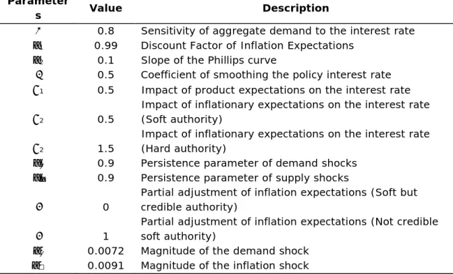
(10) ENSAYOS DE POLÍTICA ECONÓMICA – AÑO 2017 ISSN 2313-979X - Año XI Vol. II Nro. 5. III. Results III.1. Calibration of the model Table 1 shows the values of the model parameters. In general, the values are similar in both models. The magnitude of the effect of the interest rate on the product gap (𝛼 = 0.8 ) was taken from Williamson (2014) he value of the expected inflation rate impact on current inflation (𝛽1 = 0.99) was taken from Romer (2012). We set other values according our calibration process. It´s important to mention that the parameter capturing the “hardness’’ or the “softness” of the monetary authority, 𝜙2 , has two alternative values: 1.5, for a hard authority, and 0.5, for a soft one. In addition, for the case of the adaptive expectation model, we assume that: 𝑦 ∗ = 𝑟 𝑛 = 𝜋̅ = 0 (that is, the logarithms of full employment product and the natural interest rate are zero), which implies its steady state values are measured as indices equal to 1, and the inflation target is zero. Aditionally, to capture the degree of credibility of the monetary authority we consider two extreme values for λ (equation 14). First, when λ = 0, we refer to a credible authority (as regarding its plans to hit its target), and when λ=1 is considered a non-credible authority, i.e. it does not show capabilities or political motivations to hit its target. Finally, regarding the magnitude of the shocks, the standard deviation of the cyclical component of the product ( 𝜎𝑦 ) and inflation (𝜎𝜋 ) for the United States during the period 1950-2016 was considered (quarterly frequency; values obtained using the Hodrick-Prescott filter). Table 1. Model Parameters Parameter s α β1 β2 γ ϕ1. Value 0.8 0.99 0.1 0.5 0.5. ϕ2. 0.5. ϕ2 ρy ρπ. 1.5 0.9 0.9. λ. 0. λ σy σ. 1 0.0072 0.0091. Description Sensitivity of aggregate demand to the interest rate Discount Factor of Inflation Expectations Slope of the Phillips curve Coefficient of smoothing the policy interest rate Impact of product expectations on the interest rate Impact of inflationary expectations on the interest rate (Soft authority) Impact of inflationary expectations on the interest rate (Hard authority) Persistence parameter of demand shocks Persistence parameter of supply shocks Partial adjustment of inflation expectations (Soft but credible authority) Partial adjustment of inflation expectations (Not credible soft authority) Magnitude of the demand shock Magnitude of the inflation shock 65.
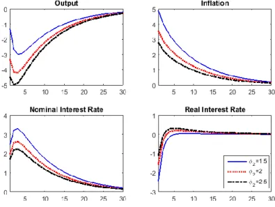
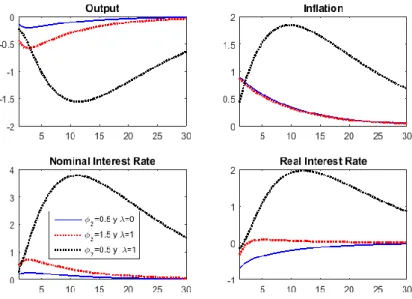
(11) III.2. Impulse-Response Results Figures 1a and 1b show the impulse-response functions of the main variables coming from a supply (or inflation) shock of positive magnitude (i. e. 𝜇𝑡𝜋 > 0). The general price level increases with respect to its steady state value. Consequently, there is a contraction of the aggregate product, as we can expect. When the inflation rate increases, the monetary authority pull up the policy interest rate, looking for close the inflation gap (the observed rate minus the target). After this shock, all the variables converge to their steady state, but a high persistence is observed in all gaps when we use the model with adaptive expectations and when a soft and not credible authority is assumed (in these case the inflation objective does not have influence in the inflation expectations, and this is observed as a slow convergence towards the steady state). This is important because the credibility of the Central Bank (i. e. that its proposals must be consistent with its actions) is a key factor to conduct the monetary policy. To observe more clearly the difference of the results when the authority is hard or soft, observe Figure 3 (Appendix B) of hyperplanes of the impulse-response functions. As the 𝜙2 coefficient increases (we are considering that 1.05 < 𝜙2 <5.05) the monetary authority manages to reduce the rate of inflation more rapidly towards its target, which is explained by the dynamics of the nominal interest rate. That is, when a Central Bank is considered hard (tough) it manages to reduce inflation quickly with a relatively low level of the interest rate; however, the product contracts more compared with the case of a soft authority. This means that the central bank faces a short run trade-off between its objectives (reducing inflation to meet the inflation target and generating greater output growth).. Figure 1. Responses to a Supply Shock (Rational Expectations and Adaptive Expectations) 1a: Responses to a Supply Shock (Rational Expectations), in percentage. 66.
(12) ENSAYOS DE POLÍTICA ECONÓMICA – AÑO 2017 ISSN 2313-979X - Año XI Vol. II Nro. 5. 1b: Responses to a Supply Shock (Adaptive Expectations), in percentage. Note: The behavior of the impulse-response functions when 𝜙2 = 0,5 and 𝜆 = 1 (Soft Authority) is on the right axis The impulse-response functions against a positive demand shock are observed in Figure 2 (2a and 2b). These figures show the results of simulating an unforeseen positive impact on aggregate demand. The effects on inflation and output lead the monetary authority to raise the nominal interest rate. In the case of adaptive expectations and not credible authority the inflation inertia is the higher. Similarly, Figure 4 (Appendix B) shows the behavior of the impulse-response functions against a supply shock. A hard Central Bank manages to reduce inflation with a lower level of the interest rate.. Figure 2. Responses to a Demand Shock (Rational and Adaptive Expectations) 2a: Responses to a Demand Shock (Rational Expectations), in percentage. 67.
(13) 2b: Responses to a Demand Shock (Adaptive Expectations), in percentage.. Note: The behavior of the impulse-response functions when 𝜙2 = 0,5 and 𝜆 = 1 (Soft Authority) is on the right axis.. IV. Welfare Analysis In this section we analyze the effects of two types of monetary authority on social welfare. The two types of authorities differ in the parameter 𝜙2 of the Taylor’s rule. A "hard" monetary authority is characterized by having a relatively large value of 𝜙2 and conversely, when this value is small then we call the monetary authority "soft". To carry out the welfare analysis, we consider the utility function of the representative consumer. First, we fix the time horizon to a sufficiently broad period, in ways that the variables converge to the steady state. This is T = 30. Second, we obtain the level of the product using the expression 𝑦𝑡 = ln 𝑌𝑡 − ln 𝑌𝑡∗ so 𝑌𝑡 = 𝑌𝑡∗ 𝑒 𝑦𝑡 . We use the assumption 𝐶𝑡 = 𝑌𝑡 ; therefore, the present value of the utilities series, our measure of welfare, is expressed in the following way:. 30. 𝑈0 = ∑ 𝛽 𝑡 𝑡=0. (𝑌𝑡∗ 𝑒 𝑦𝑡 )1−𝜎 − 1 1−𝜎. For the numerical simulations we normalize the trend product, 𝑌𝑡∗ , to the unit; the choice of σ is consistent with the calibration of 𝛼 = 0.8; so 𝜎 = 1/𝛼 = 1.25. To calculate changes in welfare, we only consider the model with adaptive expectations11, because it allows us to take into account the credibility or disbelief of the monetary authority, unlike what happens with the model with rational 11. In any case, we also did the exercise considering the model with rational expectations. The results can be seen in Table 3 of Appendix C. Certainly, the results do not change much compared to the model with adaptive expectations.. 68.
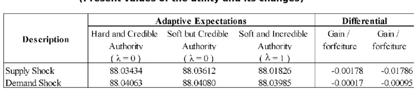
(14) ENSAYOS DE POLÍTICA ECONÓMICA – AÑO 2017 ISSN 2313-979X - Año XI Vol. II Nro. 5. expectations, where both the agents and the authority have information complete and therefore the monetary authority is always credible. Table 2 shows the results of the present value of the agent's utility series in the face of supply and demand shocks. First, when the economy faces a supply shock, the reaction of a soft but credible monetary authority generates a higher utility compared to a hard or a soft but not credible authority. In other words, if we look at the last two columns, a hard monetary authority generates a loss of welfare against a soft but credible authority equal to 0.18%; likewise, a soft but not credible authority generates a loss of welfare against a soft but credible one at 1.8%. Second, when the economy gets a demand shock, we observe that a soft but credible authority generates a welfare gain. In other words, a hard monetary authority and a soft but not credible monetary authority generate welfare losses compared to an authority that has credibility but applies the policy in a soft manner. These losses are 0.017% and 0.095%.. Table 2: Welfare analysis (Present values of the utility and its changes). Source: Authors' elaboration The numbers shown in the previous table suggest that, in the face of supply or demand shocks, a soft monetary authority is preferable, provided that it is credible, since it generates higher welfare values compared to the other types of authority. This is important in the implementation of the monetary policy, and it shows us that when it comes to announcing its monetary policy, credibility is fundamental to generate optimal results.. V. Conclusions In this paper we have used a New Keynesian Stochastic Dynamic General Equilibrium Model under two alternative setups: rational and adaptive expectations to answer this question: what is better for a society: a hard or a soft monetary authority? After solving (numerically) the model for the two types of monetary authority and facing two types of shocks, we have calculated the present value of the periodic utilities series, and based on it we were are able to answer the central question of this paper. The findings suggest that the answer depends on what might happen to the credibility of the monetary authority among economic agents if their inflation 69.
(15) expectations are configured in an adaptive manner (since the case of rational expectations excludes the possibility of disbelief in the face of an inflation target). In particular, given the occurrence of supply or demand shocks that would temporarily raise inflation, a soft authority would be the best for society if we could assume that its softness does not undermine the credibility it enjoys to drive inflation towards its objective. Otherwise, if the softness leads to the loss of credibility, a hard authority is much better judging by our measure of social welfare in summary, what seems more important is the credibility that the monetary authority deserves in terms of its willingness to do everything possible to ensure that inflation converges to the target.. VI. Bibliography Blanchard, O. J. and Kahn, C. M. (1980). The Solution of Linear Difference Models under Rational Expectations. Econometrica: Journal of the Econometric Society. 48(5):1305-1311. Cagan, P. (1956). The Monetary Dynamics of Hyperination. Studies in the Quantity Theory of Money, ed. by Milton Friedman, Chicago University Press, Chicago. Calvo, G. A. (1983). Staggered Prices in a Utility-Maximizing Framework. Journal of Monetary Economics, 12(3):383-398. Christiano, L. J. (2002). Solving Dynamic Equilibrium Models by a Method of Undetermined Coefficients. Computational Economics, 20(1-2):21-55. Davis, J. M. (2007). “News and the Term Structure in General Equilibrium.” Unpublished Manuscript. Dennis, R. (2004). Solving for Optimal Simple Rules in Rational Expectations Models. Journal of Economic Dynamics and Control, 28(8):1635-1660. Fujiwara, I., Y. Hirose, and Shintani, M. (2008). “Can News Be a Major Source of Aggregate Fluctuations? A Bayesian DSGE Approach.” IMES Discussion Paper 2008E-16. Institute for Monetary and Economic Studies, Bank of Japan. Galí, J. (2015). Monetary Policy, Inflation, and the Business Cycle: an Introduction to the New Keynesian Framework and its Applications. Princeton University Press. Hans-Werner, W. and Winkler, R. (2009). On the Non-Optimality of Information: An Analysis of the Welfare Effects of Anticipated Shocks in the New Keynesian Model. Kiel Institute for the World Economy, Kiel. Working Paper No 1497. Lubik, T. A. and Schorfheide, F. (2003). Computing Sunspots in Linear Rational Expectations Models. Working Paper 01-047, Penn Institute for Economic Research, University of Pennsylvania.. 70.
(16) ENSAYOS DE POLÍTICA ECONÓMICA – AÑO 2017 ISSN 2313-979X - Año XI Vol. II Nro. 5. Lucas, R. E. (1972). Expectations and the Neutrality of Money. Journal of Economic Theory, 4(2):103-124. Lucas, R. E. (1973). Some International Evidence on Output-Inflation Tradeoffs. The American Economic Review, 63(3):326-334. Inter-American Development Bank (2017). Macroeconomic report "Roads to grow in a new commercial world". Washington. Menz, J.O. and Vogel, L. (2009). A Detailed Derivation of the Sticky Price and Sticky Information New Keynesian DSGE Model. Technical report, DEP (Socioeconomics) Discussion Papers, Macroeconomics and Finance Series, Hamburg University. Muth, J. F. (1961). Rational Expectations and the Theory of Price Movements. Econometrica: Journal of the Econometric Society, 29(3):315-335. Nerlove, M. (1958). Adaptive Expectations and Cobweb Phenomena. The Quarterly Journal of Economics, 72(2):227-240. Romer, D. (2012). Advanced Macroeconomics. (Fourth Edition), McGraw-Hill. Rotemberg, J. J. (1982). Sticky Prices in The United States. Journal of Political Economy, 90(6):1187-1211. Sargent, T. J. and Wallace, N. (1976). Rational Expectations and The Theory of Economic Policy. Journal of Monetary Economics, 2(2):169-183. Sims, C. A. (2002). Solving Linear Rational Expectations Models. Computational Economics, 20(1):1-20. Svensson, L. E. (1997). Inflation Forecast Targeting: Implementing and Monitoring Inflation Targets. European Economic Review, 41(6):1111-1146. Taylor, J. B. (1993). Discretion versus Policy Rules in Practice. In CarnegieRochester conference series on public policy, v. 39, pp. 195-214. Walsh, C. E. (2003). Monetary Theory and Policy. (Second Edition), MIT Press. Wickens, M. (2008). Macroeconomics Theory: A dynamic general equilibrium approach. (Second Edition). Princeton University Press. Williamson, S. (2014). Macroeconomics. (Fifth Edition), Pearson. Woodford, M. (2002). Interest and Prices. Princeton University Press.. 71.
(17) VI. Annex Appendix A. Solutioning the Rational Expectations Model In this annex we develop the solution of the model with rational expectations. We rewrite equations (1), (2) and (3) as follows. 𝑦. 𝔼𝑡 (𝑦𝑡+1 |Ω𝑡 ) + 𝛼𝔼𝑡 (𝜋𝑡+1 |Ω𝑡 ) − 𝑦𝑡 − 𝛼𝑖𝑡 + 𝜀𝑡 = 0. (𝐴1). 𝛽1 𝔼𝑡 (𝜋𝑡+1 |Ω𝑡 ) + 𝛽2 𝑦𝑡 + 𝜋𝑡 + 𝜀𝑡𝜋 = 0. (𝐴2). (1 − 𝛾)𝜙1 𝔼𝑡 (𝑦𝑡+1 |Ω𝑡 ) + (1 − 𝛾)𝜙2 𝔼𝑡 (𝜋𝑡+1 |Ω𝑡 ) − 𝑖𝑡 + 𝛾𝑖𝑡−1 = 0. (𝐴3). Let 𝜃 = {𝛼, 𝛽1 , 𝛽2 , 𝛾, 𝜙1 , 𝜙2 , 𝜌𝑦 , 𝜌𝜋 , 0} be the set of model parameters of the model and let 𝑦. 𝑋𝑡 = [𝑦𝑡 , 𝜋𝑡 , 𝑖𝑡 ]′ and 𝑍𝑡 = [𝜀𝑡 , 𝜀𝑡𝜋 , 0]′ be the transposed vectors of the endogenous and exogenous variables respectively. Therefore, the matrix representation is given by:. Γ0 (𝜃)𝔼𝑡 (𝑋𝑡+1 |Ω𝑡 ) + Γ1 (𝜃)𝑋𝑡 + Γ2 (𝜃)𝑋𝑡−1 + Ψ0 (𝜃)𝑍𝑡 = 0. (𝐴4). Where: 1 0 (𝜃) Γ0 =[ (1 − 𝛾)𝜙1 0 Γ2 (𝜃) = [0 0. 0 0 0. 𝛼 𝛽1 (1 − 𝛾)𝜙2. 0 −1 0] ; Γ1 (𝜃) = [ 𝛽2 0 0. 0 1 0] ; Ψ0 (𝜃) = [0 𝛾 0. 0 1 0. 0 −1 0. −𝛼 0 ] −1. 𝑦𝑡 0 0] ; 𝑋𝑡 = [𝜋𝑡 ] 𝑖𝑡 0. The AR(1) process is represented as follows:. 𝑍𝑡 = Ψ1 (𝜃)𝑍𝑡−1 + 𝜉𝑡. (𝐴5). Where:. 𝜌𝑦 Ψ0 (𝜃) = [ 0 0. 0 𝜌𝜋 0. 𝑦 𝑦 0 𝜀𝑡 𝜇𝑡 0] ; 𝑍𝑡 = [𝜀𝑡𝜋 ] ; 𝜉𝑡 = [𝜇𝑡𝜋 ] 0 0 0. To solve the model (A4) subject to (A5) we apply the method of indeterminate coefficients method. For this we conjecture the following hypothetical solution:. 𝑋𝑡 = Φ(𝜃)𝑋𝑡−1 + Π(𝜃)𝑍𝑡 72. (𝐴6).
(18) ENSAYOS DE POLÍTICA ECONÓMICA – AÑO 2017 ISSN 2313-979X - Año XI Vol. II Nro. 5. To find the coefficients Φ(𝜃) and Π(𝜃) we advance a period and then we applied conditional expectations, taking into account that 𝔼𝑡 (𝑋𝑡 |Ω𝑡 ) = 𝑋𝑡 , from where:. 𝔼𝑡 (𝑋𝑡+1 |Ω𝑡 ) = Φ(𝜃)𝑋𝑡 + Π(𝜃) 𝔼𝑡 (𝑍𝑡+1 |Ω𝑡 ). (𝐴7). On the other hand, a period is advanced in equation (A5) and conditional expectations applied, taking into account that 𝔼𝑡 (𝑍𝑡 |Ω𝑡 ) = 𝑍𝑡 and 𝔼𝑡 (𝜉𝑡+1 ) = 0, with which it follows:. 𝔼𝑡 (𝑍𝑡+1 |Ω𝑡 ) = Ψ1 (𝜃)𝑍𝑡. (𝐴8). Substituting (A8) into (A7) yields:. 𝔼𝑡 (𝑋𝑡+1 |Ω𝑡 ) = Φ(𝜃)𝑋𝑡 + Π(𝜃) Ψ1 (𝜃)𝑍𝑡. (𝐴9). We now replace (A9) in (A4):. Γ0 (𝜃)[Φ(𝜃)𝑋𝑡 + Π(𝜃)Ψ1 (𝜃)𝑍𝑡 ] + Γ1 (𝜃)𝑋𝑡 + Γ2 (𝜃)𝑋𝑡−1 + Ψ0 (𝜃)𝑍𝑡 = 0 [Γ0 (𝜃)Φ(𝜃) + Γ1 (𝜃)]𝑋𝑡 + Γ2 (𝜃)𝑋𝑡−1 + [Γ0 (𝜃)Π(𝜃)Ψ1 (𝜃) + Ψ0 (𝜃)]𝑍𝑡 = 0. (𝐴10). Pre-multiplying the equation (A10) by; [Γ0 (𝜃)Φ(𝜃) + Γ1 (𝜃)]−1 we have:. 𝑋𝑡 = −[Γ0 (𝜃)Φ(𝜃) + Γ1 (𝜃)]−1 Γ2 (𝜃)𝑋𝑡−1 − [Γ0 (𝜃)Φ(𝜃) + Γ1 (𝜃)]−1 [Γ0 (𝜃)Π(𝜃)Ψ1 (𝜃) + Ψ0 (𝜃)] 𝑍𝑡 = 0 (𝐴11) Equating the coefficients of (28) with (A11) we deduce:. Φ(𝜃) = −[Γ0 (𝜃)Φ(𝜃) + Γ1 (𝜃)]−1 Γ2 (𝜃). (𝐴12). Π(𝜃) = −[Γ0 (𝜃)Φ(𝜃) + Γ1 (𝜃)]−1 [Γ0 (𝜃)Π(𝜃)Ψ1 (𝜃) + Ψ0 (𝜃)]. (𝐴13). To solve (A12) and (A13) a recursive method is implemented; for this we express the indexed system as follows: Φ𝑖 (𝜃) = −[Γ0 (𝜃)Φ𝑖−1 (𝜃) + Γ1 (𝜃)]−1 Γ2 (𝜃). (𝐴14). Π𝑖 (𝜃) = −[Γ0 (𝜃)Φ𝑖−1 (𝜃) + Γ1 (𝜃)]−1 [Γ0 (𝜃)Π𝑖−1 (𝜃)Ψ1 (𝜃) + Ψ0 (𝜃)]. (𝐴15). We write the system (A14) and (A15) in compact form; 𝐱 𝑖 = [Φ𝑖 (𝜃), Π𝑖 (𝜃)]′ denotes the transposed vector of unknowns and 𝐠(𝐱 𝑖−1 ) denotes the two expressions of the second member. Then we can select an arbitrary value 𝐱 0 ; which involves assigning coherent arbitrary values to Φ0 (𝜃) and Π0 (𝜃); this allows us to start the recursive 73.
(19) scheme 𝐱 𝑖 = 𝐠(𝐱 𝑖−1 ) and generate a sequence of vectors {𝐱 𝑖 = 𝐠(𝐱 𝑖−1 ) }∞ 𝑖=1 until 𝐱 𝑖 and 𝐱 𝑖−1 for some I, converge with each other, so that ‖ 𝐱 𝑖 − 𝐱 𝑖−1 ‖ = 0. The Euclidean distance or Frobenius norm is determined from the following expression:. 𝑛. 𝑛. ‖ 𝐱 𝑖 − 𝐱 𝑖−1 ‖ = √∑ ∑(𝑥𝑠𝑘,𝑖 − 𝑥𝑠𝑘,𝑖−1 ). 2. 𝑘=1 𝑠=1. Where 𝑥𝑠𝑘,𝑖 are the elements of 𝐱 𝑖 , s and k denote rows and columns respectively. Under these conditions the following optimization program is solved 12:. min ‖ 𝐱 𝑖 − 𝐱 𝑖−1 ‖ For a certain i the optimal vector 𝐱 ∗ is obtained, and therefore Φ∗ (𝜃) and Π ∗ (𝜃), which solves the previous optimization problem, which in turn also the system (A12) and (A13), and the model given by (A4). In consequence, the impulseresponse functions are given by:. 𝑋𝑡 = Φ(𝜃)∗ 𝑋𝑡−1 + Π(𝜃)∗ 𝑍𝑡 That is to say; ∗ 𝑦𝑡 𝑎11 ∗ [𝜋𝑡 ] = [𝑎21 ∗ 𝑖𝑡 𝑎31. ∗ 𝑎12 ∗ 𝑎22 ∗ 𝑎32. ∗ ∗ 𝑦𝑡−1 𝑎13 𝑏11 ∗ ∗ 𝑎23 ] [𝜋𝑡−1 ] + [𝑏21 ∗ ∗ 𝑖𝑡−1 𝑎33 𝑏31. ∗ 𝑏12 ∗ 𝑏22 ∗ 𝑏32. ∗ 𝑦 𝑏13 𝜀𝑡 ∗ 𝑏23 ] [𝜀𝑡𝜋 ] ∗ 𝑏33 0. ∗ ∗ Where 𝑎𝑠𝑘 and 𝑏𝑠𝑘 are elements of Φ∗ (𝜃) and Π ∗ (𝜃) respectively. Given the values of the parameters (Table 1), the model is solved in a spreadsheet, and it does the mechanism transparent and flexible when performing calculations and simulations.. 12. The Euclidean distance is calculated as: 2. ‖Φ𝑖 (𝜃) − Φ𝑖−1 (𝜃)‖ = √∑𝑛𝑘=1 ∑𝑛𝑠=1(𝑎𝑠𝑘,𝑖 − 𝑎𝑠𝑘,𝑖−1 ). and. 2. ‖Π𝑖 (𝜃) − Π𝑖−1 (𝜃)‖ = √∑𝑛𝑖=1 ∑𝑛𝑗=1(𝑏𝑠𝑘,𝑖 − 𝑏𝑠𝑘,𝑖−1 ) ,. so. the. distance minimization is: min {‖Φ𝑖 (𝜃) − Φ𝑖−1 (𝜃)‖ + ‖Π𝑖 (𝜃) − Π𝑖−1 (𝜃)‖}, looking for the convergence required by a model solution. Readers can acces to our spreadsheet files by requesting them at the authors address.. 74.
(20) ENSAYOS DE POLÍTICA ECONÓMICA – AÑO 2017 ISSN 2313-979X - Año XI Vol. II Nro. 5. Appendix B.. B1 (Figure 3): Observed inflation rate and inflation targets in emerging countries. Source: Elaboration of the authors with data from Latin Macro Watch (LMW), Research Department, Inter-American Development Bank (IDB). Note: The inflation data (12 months) corresponds to the growth rate of the Consumer Price Index (CPI), in monthly frequency during 2005 - 2016. The graphs are inspired by the macroeconomic report "Roads to grow in a new commercial world" prepared by the IDB, 2017.. 75.
(21) B2 (Figure 4): Responses to a Supply Shock (Rational Expectations). Note: According to the Taylor rule, 𝜙2 > 1 characterizes a hard central bank (in our simulations 1,05 ≤ 𝜙2 ≤ 5,05). The more hardness is the central bank (i.e. the bigger is 𝜙2 ), the smaller is the response of the inflation rate to a supply shock.. 76.
(22) ENSAYOS DE POLÍTICA ECONÓMICA – AÑO 2017 ISSN 2313-979X - Año XI Vol. II Nro. 5. B3 (Figure 5): Responses to a Demand Shock (Rational Expectations). Appendix C. C1 (Table 3): Welfare analysis in the model with rational expectations. Note: As in the model with adaptive expectations, the last column represents the loss of welfare of the monetary authority against the soft authority, analysis of welfare in the model with rational expectations. 77.
(23)
Figure
Documento similar
