The two sides of the model – aggregate demand and aggregate supply – collide so that equilibrium does not exist. Moreover, we model the aggregate demand side of the model to explicitly specify how the central bank can do that. Moreover, we show that even if inflation is perfectly anticipated, the solutionˆ= 0 is simply inconsistent with the equilibrium conditions on the demand side of the model.
In other words, there is a clash between the demand side and the supply side of the model. The key point of the literature from the 1970s is that this menu of choices is an illusion once expectations are adjusted. We use this form of the model for simplicity and to relate it to previous literature.
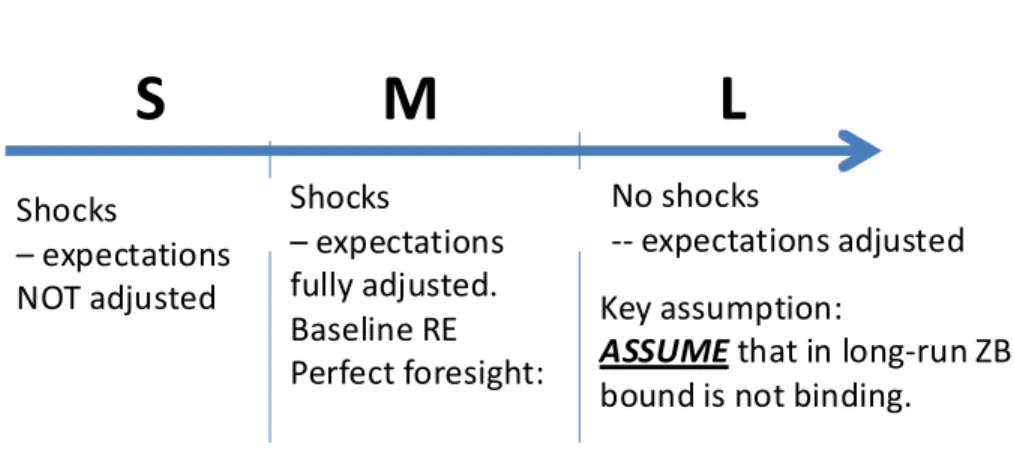
However, it is worth noting that the demand side of the model can affect the equilibrium in the case where the zero bound becomes binding. Expectations have fully adjusted in the medium and long term so that the only difference between the medium and long term is the absence of the shock in the long term. We can add money in the utility function to our framework, so that the government's choice of the nominal interest rate is then modeled by its choice of the money supply.
Before this relative price was also affected by realized inflation because inflation affected the nominal interest rate setting of the central bank.

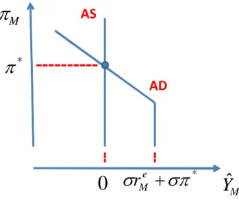
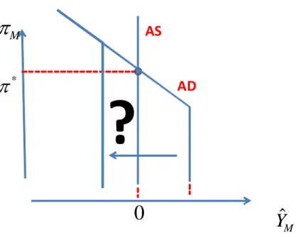
ADAS
The aggregate supply equation and the aggregate demand equation in Figure 5 point in two different directions. On the one hand, the aggregate supply equation simply states that ˆ = 0 If everyone expects the future perfectly, prices behave as if they are perfectly flexible and output is therefore potential. Meanwhile, the aggregate demand equation suggests that demand should be below its steady state, i.e. ˆ 0 For households to be willing to buy all delivered goods, the real interest rate must be sufficiently negative, but this is not possible if expected inflation is below ∗ without a negative nominal interest rate.
Obviously, demand and supply collide - no level of output and inflation satisfies both equations at the same time. What is particularly noteworthy here is that some of the political discussion reviewed in the introduction—and professional consensus—seems to be driven by an intuition derived precisely when this clash occurs, but by only using The AS equation. At the heart of the problem is the strong neutrality imposed by the AS equation in combination with a temporary shock to the AD equation that reduces demand.
Once inflation is expected, output cannot deviate from potential according to the AS equation, so there is no trade-off between inflation and. Given that some prices are fixed one period in advance (so output is demand determined in equilibrium), a critical property of the model is perfect foresight by the agents, i.e. Here we will deviate from this assumption in a way that seems quite reasonable—while still maintaining rational expectations—and show how the equilibrium is determined.
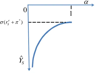
Consider our earlier assumption that a shock occurs in the short term that remains “on” in the medium term and eventually returns to a steady state in the long term. Let us now deviate from perfect foresight by assuming that there is a probability of the shock returning to a steady state in the medium term rather than in the long term. What causes the existence of the model equilibrium is that in the medium term there is no longer perfect foresight.
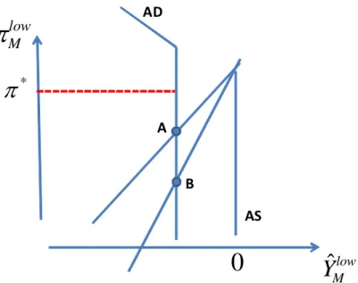
This implies that if the shock is in the low state, then the AS equation is given by Equation (25) shows that now the AS curve is no longer vertical in the medium run. This figure shows the AS and AD curves conditional on the shock remaining at its short-term value, i.e.
Y ˆ Mlow
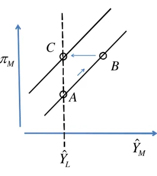
Although the level of medium-term deflation has no medium-term effect on output, it has important implications for output in the short run. In particular, we will now see that the higher the rate of deflation, the greater the drop in output in the short run. Consider the short-term solution, taking the medium-term solution derived in the last section as given.
As we saw in section 2, the static trade-off between inflation and output is the same in the short run for a given set of inflation expectations. If inflation expectations adjust completely, as is the case with perfect foresight, then there is no trade-off in the model considered so far. There is another well-defined trade-off between output and inflation in the model, which becomes very important once the nominal interest rate reaches zero.
First, we note that in the absence of a zero bound, the intertemporal trade-off between inflation and output is not significant, at least not in the medium term. Therefore, to the extent that is the only source of uncertainty, the model is deterministic in the medium and long term. The only thing that changes in the medium term with a different value∗ is the nominal interest rate required to reach equilibrium.
Remember that in the medium term we assumed that inflation expectations adjusted to policy. System 6 Suppose A2 and ≥0 Then the zero bound is not binding, the intertemporal trade-off between inflation and output in the medium term is zero, and it is given by 1+. This shows that increasing the long-term inflation target has no effect on medium-term output or inflation, it only increases the nominal interest rate in the medium term.
This is the first part of the statement that says that in the medium term there is no intertemporal trade-off. In summary, we see that while there is no intertemporal trade-off between inflation and output in the medium run, such a trade-off does exist in the short run, but its magnitude depends entirely on the extent to which short-run inflation affects the central economy will influence. bank is willing to tolerate. If a certain inflation rate is targeted in the short term, the intertemporal trade-off also disappears.
This is because with the nominal interest rate set at zero in the medium term, output is determined and given by demand. This makes it clear that intertemporal trading in the medium term is given byMeanwhile, the amount of deflation in the “low” state is given by.

ˆ lim 0
- Proof of Proposition 2
- Proof of Proposition 3
- Model
- Long-run steady state: Proof of Proposition 8
- Non-existence of medium term equilibrium: Proof of Proposition 9
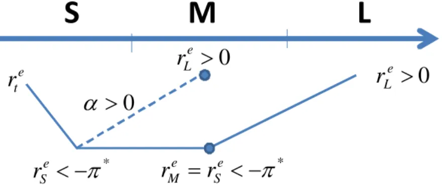
While the shock is unexpected in period=, there is perfect foresight between and The shocks in periods are identical to , i.e. it requires that be low enough, so that the representative consumer finds it preferable to consume less in the present (i.e. in the medium term) than in the future (i.e. the long term), or equivalently, to save in the medium term. Doing so reduces aggregate demand in the medium term, causing companies to lower their prices, which lowers inflation and raises the real interest rate.
That increase in real interest rates over the medium term further discourages households from consuming, leading to a collapse of the economy. Note, however, that if we are in the regular steady state with Π¯=Π∗(enΠ¯∗− 11), the higher the long-term inflation targetΠ∗the more difficult it is for the condition (32) to be satisfied, because it may need to be much lower than the medium-run equilibrium for it to cease to exist. 34;Friedman' steady state, where the medium-run equilibrium ceases to exist if the economy collapses once falls below the long-run value of , regardless of the inflation target.
So far we have only studied inflation output trading in the new classical Phillips curve model. Such a relationship can again be obtained from a log-linear approximation with an optimal pricing condition in the model described in section 2.2, but with a different assumption about pricing, e.g., when prices are scaled as in the Calvo model. Within this framework we confirm the two basic insights we have shown in the context of the previous model.
We begin by describing the long-run, medium-run, and short-run equilibria in the New Keynesian model. As in the previously discussed model, with the output Euler equation (15) and policy rule (16), the long-term inflation is ultimately equal to the long-term target, =∗in= +∗, which is positively. It is interesting that in this case and in contrast to the new classic Phillips curve, the medium-term equilibrium does not depend on the specific valueprobability of the medium-term exit from the lower bound.
However, the effect is not as dramatic as in the previous model because inflation is largely anchored by future inflation expectations, which are assumed here to be unaffected. However, these expressions make it clear that a negative value of has even stronger adverse effects on output and inflation in the short run than it does in the medium run. While the equilibrium in the basic version of the New Keynesian model exists even in the presence of a persistent situation.
Again, the temporary increase in the inflation target may moderate the negative impact of the shock in the model. The nonlinear model described in the text is repeated here for convenience using (13) to eliminate and.