A multidimensional dynamical approach to iterative methods with memory
22
0
0
Texto completo
(2) Theorem 1. Let ψ be an iterative method with memory that generates a sequence {xk } of approximations to the root α, and let this sequence converges to α. If there exist a nonzero constant η and nonnegative numbers ti , i = 0, 1, . . . , m, such that the inequality m ! |ek+1 | ≤ η |ek−i |ti i=0. holds, then the R-order of convergence of the iterative method ψ satisfies the inequality OR (ψ, α) ≥ s∗ , where s∗ is the unique positive root of the equation sm+1 −. m ". ti sm−i = 0.. i=0. In this paper, we transform iterative methods with memory in discrete dynamical systems (Section 2). In the following, we consider the study of some new iterative schemes with memory of different orders of convergence: the Secant method (Section 3), the modified Steffensen’s method (Section 4), the modified Traub’s method (Section 5) and, finally, a modified parametric family with memory (Section 6), applied on 2-degree polynomials. In this last case, as we have a family depending on a parameter some bifurcation diagrams are built. The existence of chaos can be observed for certain values of the parameter. 2. Iterative methods with memory as discrete dynamical systems As it was stated in the Introduction, the dynamical behavior of the operators associated to numerical methods is an efficient tool for analyzing the stability of the methods. In this section we built the discrete dynamical system associated to an iterative methods with memory in order to carry out its dynamical study. The expression of an iterative method with memory, which uses two previous iterations to calculate the following estimation, is xk+1 = g(xk−1 , xk ), k ≥ 1, where x0 and x1 are the initial estimations. A fixed point of this method will be obtained when not only xk+1 = xk , but also xk−1 = xk . In order to obtain them, we define the fixed point function G : R2 −→ R2 by means of: G (xk−1 , xk ). = =. (xk , xk+1 ), (xk , g(xk−1 , xk )), k = 1, 2, . . . ,. being x0 and x1 the initial estimations. This definition can be extended in a natural way to adapt it to iterative schemes with memory that use more than two previous iterations per step. As (xk−1 , xk ) is a fixed point of G if G (xk−1 , xk ) = (xk−1 , xk ), then, xk+1 = xk and xk−1 = xk . So, the mentioned conditions are satisfied. We have defined a discrete dynamical system in the plane from the function G : R2 → R2 , given by G(z, x) = (x, g(z, x)) where g is the operator of the iterative method with memory. Fixed points (z, x) of G satisfy z = x and x = g(z, x). In the following we recall some basic dynamical concepts. Definition 1. If a fixed point (z, x) of operator G is different from (r, r), where r is a zero of f , it is called strange fixed point. Definition 2. Let G : R2 → R2 be a vectorial function. The orbit of a point x̄ ∈ R2 is defined as the set of successive images of x̄ by the vector function, {x̄, G(x̄), . . . , Gm (x̄), . . .}. 2.
(3) The dynamical behavior of the orbit of a point of R2 is classified depending on its asymptotical behavior. Definition 3. A point x∗ ∈ R2 is a k-periodic point if Gk (x∗ ) = x∗ and Gp (x∗ ) '= x∗ , for p = 1, 2, . . . , k − 1. The stability of fixed points for multivariable nonlinear operators, see for example [20], satisfies the following statements: Theorem 2. Let G from Rn to Rn be C 2 . Assume x∗ is a k-periodic point. Let λ1 , λ2 , . . . , λn be the eigenvalues of G# (x∗ ). a) If all the eigenvalues λj have |λj | < 1, then x∗ is attracting. b) If one eigenvalue λj0 has |λj0 | > 1, then x∗ is unstable, that is, repelling or saddle. c) If all the eigenvalues λj have |λj | > 1, then x∗ is repelling. In addition, a fixed point is called hyperbolic if all the eigenvalues λj of G# (x∗ ) have |λj | '= 1. In particular, if there exist an eigenvalue λi such that |λi | < 1 and an eigenvalue λj such that |λj | > 1, the hyperbolic point is called saddle point. Then, if x∗ is an attracting fixed point of function G, its basin of attraction A(x∗ ) is defined as the set of pre-images of any order such that # $ A(x∗ ) = x(0) ∈ Rn : Gm (x(0) ) → x∗ , m → ∞ .. The set of the different basins of attraction define the dynamical plane of the system. The dynamical plane of a method is built by iterating a mesh of points and painting them in different colors depending on the attractor they converge to. All the methods that we analyze in this paper do not use the derivative of function f , so it is not possible to establish a scaling theorem (see [21]). Therefore, to accomplish our study we consider the quadratic polynomial p(x) = x2 − 1. So, the fixed point function G is a rational function. In the following sections we carry out our study of the different methods analyzing their dynamical behavior and their local convergence. 3. Secant method We begin by studying the best known iterative scheme with memory, the Secant method, whose iterative expression is f (xk )(xk − xk−1 ) xk+1 = xk − , k ≥ 1. f (xk ) − f (xk−1 ) This method has superlinear convergence in a neighborhood of a simple zero of f , and the proof can be found in [19]. Let us apply the extended dynamical concepts to the Secant method with memory. In this case, we denote by Sf the fixed point function associated to Secant method on f (x). The associate fixed point operator is a function of two variables: the last one, xk (denoted by x) and the previous one xk−1 denoted by z. So, % & % & p(x)(x − z) 1 + xz Sp (z, x) = x, x − = x, . p(x) − p(z) x+z Let us notice that this operator is not defined for z = −x. Now, we analyze the stability of the method by studying the asymptotic behavior of the fixed points.. Lemma 1. The only fixed points of the operator associated to Secant iterative method on quadratic polynomial p(x) correspond to its roots, x = z = ±1, being both attracting. Proof: By solving the equation. Sp (z, x) = (z, x) ⇔ x = z = ±1,. we find that that the only fixed points are (z, x) = (−1, −1) and (z, x) = (1, 1). To study their behavior, we will use Theorem 2: 3.
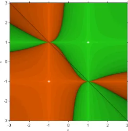
(4) • Let us consider (z, x) = (1, 1). The Jacobian matrix of Sp (z, x) at this point is Sp# (1, 1). =. %. 0 0. 1 0. &. and the eigenvalues of Sp# (1, 1) are λ1 = λ2 = 0. • If (z, x) = (−1, −1), the eigenvalues of the associated Jacobian matrix are also λ1 = λ2 = 0. And then, by applying Theorem 2, (1, 1) and (−1, −1) are attracting fixed points of Secant method.. !. In Figure 1, the dynamical plane associated with Secant method is showed, being x and z real. Variable x is plotted in abscissas axis and z in the ordinates one. This plane has been generated by slightly modifying the routines described in [22]. In them, a mesh of 400 × 400 points has been used, 40 has been the maximum number of iterations involved and 10−3 the tolerance used in the stopping criterium (the absolute error). Then, if an starting point (x, z) of this mesh converges to one of the roots of the polynomial (white stars placed on the line x = z), it is painted in the color assigned to the root which has converged to. The color used is brighter when the number of iterations is lower. If it reaches the maximum number of iterations without converging to any of the roots, it is painted in black. It can be observed in Figure 1 that both roots of p(x) have their respective basins of attraction forming a symmetric division of the real plane into two parts. 4. Modified Steffensen method with memory It is well known that Steffensen method has second-order of convergence and it is derivative-free, with the iterative expression f (xk ) xk+1 = xk − , k ≥ 0, f [xk , wk ] being wk = xk + f (xk ) and denoting by f [·, ·] the usual first-order divided difference. 4.1. Design and local convergence If a damping parameter γ is considered in the definition of wk = xk + γf (xk ), then the order of convergence f ## (α) is held and the error equation is ek+1 = (1 + f # (α)γ)c2 e2k + O(e3k ), where c2 = . This expression of the 2f # (α) error equation is the key for transforming the iterative scheme in other one with memory: if we could consider 1 γ=− # , the order of the scheme would be at least three; as it has no sense to use the root of function f , we f (α) 1 can estimate it by using the two previous iterations, γ = − , getting a scheme with memory by the use f [xk , xk−1 ] of the previous iteration xk−1 as in Secant method. Let us remark that this estimation is the same as the obtained by approximating the nonlinear function by its first-degree Newton interpolation polynomial f (x) ≈ N1 (xk , xk−1 ) 1 and then getting γ = − # . The final iterative expression of the method, that will be called MST is N1 (xk , xk−1 ) given by γk. =. wk. =. xk+1. =. −1 , f [xk−1 , xk ] xk + γk f (xk ), f (xk ) xk − , k = 1, 2, . . . f [xk , wk ]. where x0 , x1 are the initial estimations. The local convergence of this scheme is analyzed in the following result. 4. (1).
(5) Theorem 3. Let α be a simple zero of a sufficiently differentiable function f : D ⊂ R → R in an open interval D. If√x0 and x1 are sufficiently close to α, then the order of convergence of method with memory (1) is at least 1 + 2, being its error equation ek+1 = c22 ek−1 e2k + O4 (ek−1 ek ), f (k) (α) , k ≥ 2 and O4 (ek−1 ek ) indicates that the sum of the k!f # (α) and ek in the rejected terms of the development is at least 4.. where ek−1 = xk−1 − α, ek = xk − α, ck = exponents of ek−1. Proof: By using Taylor series expansions, f (xk ) and f (xk−1 ) can be expressed as ' ( f (xk−1 ) = f # (α) ek−1 + c2 e2k−1 + c3 e3k−1 + O(e4k−1 ), ' ( f (xk ) = f # (α) ek + c2 e2k + c3 e3k + O(e4k ). Then. γk. = =. and wk − α. = =. ek−1 − ek f (xk−1 ) − f (xk ) ) * ) * 1 ' −1 + c2 ek−1 + c2 ek + c3 − c22 e2k−1 + c3 − c22 e2k # f (α) ) * ( + c3 − 2c22 ek ek−1 + O3 (ek−1 ek ). −. ek + γk f (xk ) ) * c2 ek−1 ek − c22 − c3 ek−1 e2k + (c3 − c22 )e2k−1 ek + O4 (ek−1 ek ).. So, by using the previous developments, it can be stated that f [xk , wk ] = = and. f (xk ) − f (wk ) xk − w k ) * f # (α) 1 + c2 ek + c22 ek−1 ek + c3 e2k + O3 (ek−1 ek ). f (xk ) f [xk , wk ]. =. ek − c22 ek−1 e2k + O4 (ek−1 ek ).. ek+1. =. ek −. =. c22 ek−1 e2k + O4 (ek−1 ek ).. Then, f (xk ) f [xk , wk ]. As the lower term of the error equation is c22 ek−1 e2k , by using Theorem 1, we have that the √ unique positive root of polynomial p2 − 2p − 1 gives us the R-order of the method, being in this case p = 1 + 2. ! 4.2. Dynamical study The fixed point operator resulting from applying this scheme on p(x) = x2 − 1 is a function of two variables: the last iteration, xk (denoted by x) and the previous one xk−1 denoted by z. So, % & z + x(2 + xz) Stp (z, x) = x, . 1 + x2 + 2xz Let us remark that this operator is not defined on the curve 1 + x2 + 2xz = 0. To study the stability of the method we will analyze the asymptotic behavior of the fixed points. Lemma 2. The fixed points of the operator Stp (z, x) are (z, x) = (1, 1) and (z, x) = (−1, −1), being both attracting, and (z, x) = (0, 0), which is a saddle point. 5.
(6) Proof: The fixed points are obtained by solving the equation Stp (z, x) = (z, x) . x(xz + 2) + z = x, that is z = x and (−1 + x2 )2x = 0. So, (z, x) = (1, 1), x2 + 2xz + 1 (z, x) = (−1, −1) and (z, x) = (0, 0) are fixed points of Stp (z, x). To study their asymptotic behavior, we use Theorem 2: Then, we find that z = x and. • Let us consider z = x = 1: the eigenvalues of St#p (1, 1) are λ1 = λ2 = 0, then (z, x) = (1, 1) is attracting. • If z = x = −1, the eigenvalues of St#p (−1, −1) are λ1 = λ2 = 0; so, (z, x) = (−1, −1) is also an attracting fixed point. • (z, x) = (0, 0) is also a fixed point of operator Stp (z, x); the eigenvalues of St#p (0, 0) are λ1 = 1 − √ λ2 = 1 + 2; then, it is a saddle point.. √. 2 and. ! In Figure 2, the dynamical plane associated with modified Steffensen method with memory on p(x) is shown, being x and z real. Let us notice that, being very similar to Figure 1, brighter colors in Figure 2 reveal quicker convergence and in both cases there exists convergence to the roots for any initial estimation in the real plane. 5. Modified Traub’s scheme with memory Let us consider third-order Traub’s scheme [1] with the iterative expression yk. =. xk+1. =. f (xk ) , f # (xk ) f (yk ) yk − # , k ≥ 0, f (xk ) xk −. that is obtained by composing Newton’s method with itself but holding the derivative in the second step as in the first one. 5.1. Design and local convergence If we transform this multipoint method in a derivative-free one by simply substituting f # (xk ) ≈ f [xk , wk ], where wk = xk + γf (xk ) we get yk. =. xk+1. =. f (xk ) , f [xk , wk ] f (yk ) yk − , k ≥ 0, f [xk , wk ] xk −. then the order of convergence is held and the error equation is ek+1 = (1 + f # (α)γ)(2 + f # (α)γ)c22 e3k + O(e4k ), f ## (α) being c2 = . From this expression there exist two possibilities for transforming the iterative scheme in 2f # (α) 1 2 other one with memory: γ = − # or γ = − # , in both cases the order of the scheme would be at f (α) f (α) 1 least four; as in the previous section, we estimate γ by using the two previous iterations, γ1k = − f [xk , xk−1 ] 2 or γ2k = − , getting a scheme with memory by the use of the previous iteration xk−1 as in Secant f [xk , xk−1 ] 6.
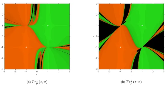
(7) method, whose iterative expression is, γ 1k. =. wk. =. yk. =. xk+1. =. 1 2 (γ2k = − ) f [xk , xk−1 ] f [xk , xk−1 ] xk + γ1k f (xk ) (wk = xk + γ2k f (xk )) f (xk ) xk − , f [xk , wk ] f (yk ) yk − , k ≥ 0. f [xk , wk ] −. (2). The local convergence of the resulting schemes is analyzed in the following result. Theorem 4. Let α be a simple zero of a sufficiently differentiable function f : D ⊂ R → R in an open interval D. If x0 and x1 are sufficiently close to α, then the order of convergence of method with memory (2) is at √ * 1) least 3 + 13 . The error equation, depending on the estimation of the damping parameter used, γ1k = 2 1 2 − or γ2k = − , is f [xk , xk−1 ] f [xk , xk−1 ] ek+1 = c32 ek−1 e3k + O5 (ek−1 ek ), or. ek+1 = −2c32 ek−1 e3k + O5 (ek−1 ek ),. respectively.. Proof: By using Taylor series expansions of higher order than the used in the proof of Theorem 3 (with γ1 ), we obtain yk. = =. f (xk ) f [xk , wk ] ) * ) * 2 c2 ek−1 e2k + 2c2 c3 − 2c32 ek−1 e3k + c2 c3 − c32 e2k−1 e2k + O5 (ek−1 ek ), xk −. then, the Taylor development of the quotient of the last step yields f (yk ) f [xk , wk ]. =. ) * ) * c22 ek−1 e2k + 2c2 c3 − 3c32 ek−1 e3k + c2 c3 − c32 e2k−1 e2k + O5 (ek−1 ek ),. and the error equation results. ek+1. =. c32 ek−1 e3k + O5 (ek−1 ek ).. 2 As the lower error term is c32 ek−1 e3k , by using Theorem 1) the unique √ * positive root of polynomial p − 3p − 1 gives 1 us the R-order of the method, being in this case p = 2 3 + 13 and the result is proven. In a similar way, the result from γ2 can be stated. !. 5.2. Dynamical study Now, we analyze the dynamics of both schemes, called M T M1 and M T M2 , respectively. The associate fixed point operator is, in each case, T rp1. (z, x). =. T rp2 (z, x). =. !. x,. " 4 # " # " # " #$ 3x + 6x2 − 1 z 3 + 3x x4 + 6x2 + 1 z 2 + x6 + 12x4 + 9x2 + 2 z + x 3x4 + 2x2 + 3. , (x2 + 2xz + 1)3 ! " # " # " # " #$ 3x4 + 6x2 − 1 z 3 − 3x x4 − 6x2 − 3 z 2 + x6 − 6x4 + 21x2 + 8 z − x x6 − 6x4 + 13x2 − 16 x, , 8(xz + 1)3. being x the last iteration and z the previous one. So, to analyze the stability of the schemes we will study the asymptotic behavior of the fixed points. In Figure 3 the dynamical planes associated to T rp1 (z, x) and T rp2 (z, x) can be seen. Let us observe that the behavior of the first one is better, being wider the basins of attraction of the roots and smaller the areas of no convergence. Indeed, let us remember that the asymptotic error of M T M2 method is the double of the one of M T M1 . This is the reason why we focus our attention on fixed point operator T rp1 (z, x), although all the calculations can be made in a similar way for T rp2 (z, x). 7.
(8) Lemma 3. The fixed points of the operator associated to M T M1 on quadratic polynomial p(x) are: a) Points (1, 1) and (−1, −1) associated to the roots, being both attracting, b) The strange fixed point (z, x) = (0, 0) which is a saddle point. Proof: The fixed points are obtained by solving the equation T rp1 (z, x) = (z, x) that is, z. =. x. =. x) * ) * ) * ) * x 3 + 2x2 + 3x4 + 2 + 9x2 + 12x4 + x6 z + 3x 1 + 6x2 + x4 z 2 + −1 + 6x2 + 3x4 z 3 (1 + x2 + 2xz). or. 3. ,. −4(−1 + x)x(1 + x)(1 + 2x2 + 5x4 ) = 0.. It is clear that z = x = ±1 and z = x = 0 satisfy the previous equation. Moreover, the factor 1 + 2x2 + 5x4 is greater than zero for any real x. So, they are the only fixed points. We analyze now their stability by studying the absolute value of the eigenvalues of the Jacobian matrix associated to the fixed point operator of the method on these fixed points. From Theorem 2: #. a) The eigenvalues of T rp1 (1, 1) are λ1 = λ2 = 0, so z = x = 1 is attracting. Moreover, the eigenvalues of # T rp1 (−1, −1) are λ1 = λ2 = 0; so, z = x = −1 is also an attracting fixed point. √ * √ * ) ) # b) T rp1 (0, 0) has as eigenvalues λ1 = 12 3 − 17 and λ2 = 12 3 + 17 ; so, it is a saddle point. !. 6. Modified parametric family with memory The fourth-order parametric family under study was presented in [23] as an efficient class to estimate the solution of nonlinear systems of equations. Its iterative expression in the scalar case is yk. =. tk. =. xk+1. =. f (xk ) , f # (xk ) f (yk ) + θf (xk ) xk − , f # (xk ) f (tk ) + f (yk ) + θf (xk ) xk − , k = 1, 2, . . . f # (xk ) xk − θ. and its local order of convergence is three, being fourth-order for θ = ±1, under standard conditions. We denote this family by HMT. 6.1. Design and local convergence In a similar way as it has been made in Traub’s scheme, we replace the derivative in HMT class by a parametric divided difference of first order, f # (xk ) ≈ f [xk , wk ], being wk = xk + γf (xk ). yk. =. tk. =. xk+1. =. f (xk ) , f [xk , wk ] f (yk ) + θf (xk ) xk − , f [xk , wk ] f (tk ) + f (yk ) + θf (xk ) xk − , k = 1, 2, . . . f [xk , wk ] xk − θ. 8.
(9) Then, the third-order of convergence is held and the error equation is ek+1 = −(2 + f # (α)γ)(θ − 1)(θ + f # (α)γ + f ## (α) 1)c22 e3k + O(e4k ), where c2 = . Let us notice that the possibility of getting fourth-order of convergence is 2f # (α) also held for θ = 1, but not for θ = −1. To transform the iterative family in other one with memory increasing 2 the order of convergence we need that γ = − # ; as in the previous section, we estimate γ by using the two f (α) 2 previous iterations, γk = − , getting a scheme with memory by the use of the previous iteration xk−1 , f [xk , xk−1 ] whose iterative expression is γk. =. wk. =. yk. =. tk. =. xk+1. =. 2 f [xk , xk−1 ] xk + γk f (xk ) f (xk ) xk − θ , f [xk , wk ] f (yk ) + θf (xk ) xk − , f [xk , wk ] f (tk ) + f (yk ) + θf (xk ) xk − , k = 1, 2, . . . f [xk , wk ] −. (3). The local convergence of the resulting scheme, called M HM T , is analyzed below. Theorem 5. Let α be a simple zero of a sufficiently differentiable function f : D ⊂ R → R in an open interval D. If x0 and x1 are sufficiently close to α, then the order of convergence of method with memory (3) is at least √ * 1) 3 + 13 . The error equation is 2 ) ) ** ek+1 = −2 (−1 + θ)2 c32 ek−1 e3k + O5 (ek−1 ek ), where cj =. 1 f (j) (α) , j = 2, 3, . . . However, if θ = 1, the error equation is j! f # (α). being the local order 2 +. √. ek+1 = −4c52 e2k−1 e4k + O7 (ek−1 ek ), 6 in this case.. Proof: By using Taylor series expansions of higher order than the used in previous results (but with γk = 2 − f [xk−1 ,xk ] ), we obtain yk − α. =. ek − θ. f (xk ) f [xk , wk ]. ) * = (1 − θ)ek − θc2 e2k + 2θc22 ek−1 e2k + 2θc2 −c22 + c3 e2k−1 e2k ) + (θc2 c3 − θc4 )) e4k + O5 (ek−1 ek ),. then, the Taylor development of the second step is tk − α. = =. f (yk ) + θf (xk ) f [xk , wk ] ) * ) * −(−1 + θ)2 c2 e2k − 2 (−1 + θ)c22 ek−1 e2k + (−1 + θ)θ −2c22 + (−2 + θ)c3 e3k ) * +2(−1 + θ)c2 c22 − c3 e2k−1 e2k + 2θ(−4 + 3θ)c32 ek−1 e3k ) ) * * + −θ2 c32 + 1 − 5θ2 + 3θ3 c2 c3 − (−1 + θ)4 c4 e4k + O5 (ek−1 ek ) ek −. and finally the error equation yields ek+1. =. ) * −2 (−1 + θ)2 c32 ek−1 e3k + O5 (ek−1 ek ).. By using Theorem 1 the )unique root of polynomial p2 − 3p − 1 gives us the R-order of the method, √ positive * 1 being in this case p = 2 3 + 13 . In the particular case θ = 1, it can be checked that the error equation is ek+1 = −4c52 e2k−1 e4k + O7 (ek−1 ek ) and the polynomial whose positive root gives us the local order is p2 − 4p − 2, √ that yields p = 2 + 6. ! 9.
(10) 6.2. Dynamical study Now, we analyze the dynamics of the operator associated to the new method M HM T . The associate fixed point operator is, Hpθ. (z, x). =. !. $ " # & " −1 + x2 (x + z) %" 2 #3 4 2 #2 x, x − −1 + x q1 (z, x, θ) + 16(1 + xz) q2 (z, x) + −1 + x q3 (z, x, θ) , 64(1 + xz)6 (2 + 2xz). ) * 4 3 2 2 2 where q1 (z, x, θ) = θ4 (x + z)6 −)8θ3 (x + z)4 (1 + xz), q (z, x) = 8 + x + 10xz − 2x z − z + 5x −1 + z 2 * ) * and q3 (z, x, θ) = −32θ(1 + xz)3 −2 + x2 + z 2 + 8θ2 (x + z)2 (1 + xz)2 −4 + 3x2 + z 2 . So, to analyze the stability of the schemes we study the asymptotic behavior of the fixed points. Lemma 4. The fixed points of the operator associated to M HM T on quadratic polynomial p(x) are: a) Points (1, 1) and (−1, −1) associated to the roots, being both attracting.. b) The origin (z, x) = (0, 0), which is an attracting fixed point for −4 < θ < −2. ) * ) * ) * c) The polynomial m(x) = 2+θ+ 9 − 2θ2* x2 + 17 − 3θ + 2θ2 + 2θ3 x4 +* 18 + 4θ2 − 4θ3 − θ4 x6 + ) real roots of * ) ) 12 + 3θ − 4θ2 + 3θ4 x8 + 5 − 2θ2 + 4θ3 − 3θ4 x10 + 1 − θ + 2θ2 − 2θ3 + θ4 x12 , whose number varies depending on the range of parameter θ: there are two real saddle points if θ < −2, none if −2 ≤ θ < 6.66633, two non-hyperbolic points if θ = 6.66633 and four (two saddle and two repulsive points) if θ > 6.66633. Proof: The fixed points are obtained by solving the equation Hpθ (z, x) = (z, x) , that is, z = x and −. 1 (−1 + x)x(1 + x)m(x) = 0. (1 + x2 )7. It is clear that the points (1, 1) and (−1, −1) satisfy the previous equation and both eigenvalues of the associate Jacobian matrix on them) are null,√so they are attracting. Obviously, (0, 0)√is also a fixed *point; its associated * ) eigenvalues are λ1 = 14 4 + θ − 32 + 16θ + θ2 and λ2 = 14 4 + θ + 32 + 16θ + θ2 . It can be checked that, being θ real, |λ1 | < 1 and |λ2 | < 1 if and only if −4 < θ < −2. So, when parameter θ is taken in this interval, the origin is an attracting strange fixed point. The rest of strange fixed points will be the roots of the twelfth-degree polynomial m(x), denoted by ri , i = 1, 2, . . . , 12. We analyze now their stability by studying the absolute value of the eigenvalues of the Jacobian matrix associated to the fixed point operator of the method on these fixed points. It can be checked that, when θ < −2, only two roots of m(x), r1 and r2 , are real and the absolute value of the eigenvalues of the Jacobian matrix associated to the fixed point operator on them coincide and they can be seen in Figure 4a. It can be observed that one of the eigenvalues is always lower than one (in absolute value) and the other one remains higher than one; so, by applying Theorem 1, both strange fixed points are saddle points. Besides, when −2 ≤ θ < 6.66633, none of the roots of m(x) is real. Moreover, when θ = 6.66633, both r1 and r3 are real; their associated eigenvalues coincide, being λ1 = 1 and λ2 = 0.934034. So, both points are not hyperbolic. Finally, if θ > 6.66633, roots r1 to r4 are real and the stability of r1 and r4 coincide, as well as the stability of r2 and r3 (see Figures 4b and 4c). ! The behavior of these fixed points is reflected in the dynamical planes; it can be observed that the roots of the polynomial and also the possible attracting fixed points are located on the bisectrix z = x of the plane. The stable behavior of the origin can be seen at Figure 5b, where the basin of attraction of point (0, 0) is plotted in blue. Moreover, in Figures 5c, 5d and 5e only the basins of attraction of the solutions are found but the second one shows wider regions of stability; let us remark that this picture corresponds to the value of θ that provides higher order of convergence of the family. Finally, a highly unstable behavior can be observed in Figures 5a and 5f, where big black areas of no convergence to the roots appear and the basins of attraction of the roots are very narrow. Let us remark that, although the dynamics of the family is, in general, very stable, for particular values of the parameter there exist attracting fixed points different from the solutions of the problem. In the following section we see how this stability varies in terms of the parameter. 10.
(11) In order to analyze the behavior of the whole parametric family, it is frequent to use a bifurcation diagram, called Feigenbaum diagram, to study the changes of behavior of a fixed point, depending on the values of parameter θ. These bifurcations can show a change of stability of the fixed points, or even doubling-period bifurcations (where the periodic or fixed point splits into a periodic orbit with a period that duplicates the previous one), pitch-fork bifurcations (where the fixed point changes the stability and also appears a periodic orbit which holds the previous stability of the fixed points), etc. Summarizing, these kind of diagrams show us the way from regularity to chaos, if it exists. This kind of tools has been used to analyze the Henon map, that is also defined in the real plane, obtaining period doubling bifurcation an even chaotic behavior depending on the value of the involved parameter (see, for example, [24] [25] or [26]). 6.3. Bifurcation diagrams In this section we present the bifurcation diagrams of the map associated to MHMT family on quadratic polynomial p(x), by using as a starting point each one of the strange fixed points of the map and observing the ranges of the parameter θ where changes of stability or other behaviors happen. This allows us to check the studied dependence of the stability of these points on the parameter and also to find numerically some strange attractors. By using the strange fixed point (0, 0) as initial estimation, a Feigenbaum diagram can be seen in Figure 6. Let us remark in this case that it fully coincides with the stability of this fixed point, stated in Lemma 4; that is, (0, 0) is an attracting fixed point for θ ∈] − 4, −2[. Out of this interval iterations (points in blue color) tend to one of the roots, -1 and 1. To draw these Feigenbaum diagrams, 500 elements of the orbit of each strange fixed point are calculated, plotting the last 400, for each value of parameter θ (after a partition of the analyzed interval in 3000 subintervals). To do this, related to strange fixed points ri , i = 1, 2, . . . , 12, the change of variables t2 = s has been used in polynomial m(t), getting a sixth-order polynomial whose roots are called si , i = 1, 2, . . . , 6. Obviously, roots √ ri , i = 1, 2, . . . , 12, of m(t) are obtained as rj = ± si . To avoid unnecessary repetitions, we do not show the Feigenbaum diagrams of all the strange fixed points. It has been checked that the orbits of these fixed points depend on the stability of the origin (some of them tend to (0, 0) for θ ∈] − 4, −2[), but mostly tend to the roots of p(x). However, some details of these bifurcation diagrams must be calculated, as it seems chaotic behavior is observed in some Figures 7 and 8. Specific regions of (θ, x)-planes are plotted in the bifurcation diagrams (Figure 9). In order to better understand the behavior of family MHMT with memory, we plot in (z, x)-space the iteration of operator Hpθ (z, x), for values of parameter θ in the blue region of Figure 9b. So, two symmetric attractors have been found, (see Figure 10). The way these pictures have been obtained is the following: fixing the value of parameter θ, 10000 different initial estimations have been taken in rectangles [−0.66, −0.62] × [−0.66, −0.62] (Figure 10a) and [0.62, 0.66] × [0.62, 0.66] (Figure 10b). The method has been used on each of them, plotting one point per iteration. The resulting images show that two attracting orbits appear and it can be observed that starting points inside and outside the orbit tend to it. However, the set of initial estimations that belong to their respective basins of attraction is very reduced, as well as the interval of real values of θ that induces this behavior. 7. Conclusions In this paper, we have adapted some tools of the dynamical analysis of multivariate real discrete problems to analyze the stability of the fixed points of iterative methods with memory on quadratic polynomials. As far as we know, this kind of analysis has not been performed before on iterative methods with memory for solving nonlinear equations. From the well-known Secant method as initial inspiration, we have designed new methods with memory from Steffensen’ or Traub’s schemes (in the last case we have previously transformed it in a derivative-free method), as well as a parametric family of iterative procedures of third- and fourth-order of convergence. Our statements, based on consistent discrete dynamics results and also on Feigenbaum diagrams of the family, allow us to select the most stable elements of the class and to find those that present convergence to other points different from the solution of our problem or even chaotic behavior. Acknowledgments: The authors thank to the anonymous referees for their suggestions to improve the readability of the paper. [1] J.F. Traub, Iterative methods for the solution of equations, Chelsea Publishing Company, New York, 1982. 11.
(12) [2] M. Petković, B. Neta, L. Petković, J. Džunić, Multipoint methods for solving nonlinear equations, Academic Press, 2013. [3] X. Wang, T. Zhang, Efficient n-point iterative methods with memory for solving nonlinear equations, Numerical Algorithms (2015), doi: 10.1007/s11075-014-9951-8. [4] J. P. Jaiswal, Solving Nondifferentiable Nonlinear Equations by New Steffensen-Type Iterative Methods with Memory, Mathematical Problems in Engineering, Volume 2014 (2014), Article ID 795628, 6 pages. [5] T. Lotfi, F. Soleymani, S. Shateyi, P. Assari, F. Khaksar Haghani, New Mono- and Biaccelerator Iterative Methods with Memory for Nonlinear Equations, Abstract and Applied Analysis, Volume 2014 (2014), Article ID 705674, 8 pages. [6] A. Cordero, T. Lotfi, P. Bakhtiari, J.R. Torregrosa, An efficient two-parametric family with memory for nonlinear equations, Numerical Algorithms 68 (2015) 323–335. [7] S. Amat, S. Busquier, C. Bermúdez, S. Plaza, On two families of high order Newton type methods, Applied Mathematic Letters 25 (2012) 2209–2217. [8] S. Amat, S. Busquier, S. Plaza, Chaotic dynamics of a third-order Newton-type method, Journal of Mathematical Analysis and Applications 366 (2010) 24–32. [9] S. Amat, S. Busquier, Á. A. Magreñán, Reducing Chaos and Bifurcations in Newton-Type Methods, Abstract and Applied Analysis, Volume 2013 (2013), Article ID 726701, 10 pages http://dx.doi.org/10.1155/2013/726701. [10] D. K. R. Babajee, A. Cordero, F. Soleymani, J.R. Torregrosa: On improved three-step schemes with high efficiency index and their dynamics, Numerical Algorithms 65(1) (2014) 153–169. [11] C. Chun, B. Neta, J. Kozdon, M. Scott, Choosing weight functions in iterative methods for simple roots, Applied Mathematics and Computation 227 (2014) 788–800. [12] A. Cordero, J.R. Torregrosa, P. Vindel, Dynamics of a family of Chebyshev-Halley type methods, Applied Mathematics and Computation 219 (2013) 8568–8583. [13] A. Cordero, J. Garcı́a, J.R. Torregrosa, M.P. Vassileva, P. Vindel, Chaos in King’s iterative family, Applied Mathematic Letters 26 (2013) 842–848. [14] Á. A. Magreñán, Estudio de la dinámica del método de Newton amortiguado (PhD Thesis), Servicio de Publicaciones, Universidad de La Rioja, 2013. http://dialnet.unirioja.es/servlet/tesis?codigo=38821. [15] Á. A. Magreñán, Different anomalies in a Jarratt family of iterative root-finding methods, Applied Mathematics and Computation 233 (2014) 29–38. [16] B. Neta, C. Chun, M. Scott, Basins of attraction for optimal eighth order methods to find simple roots of nonlinear equations, Applied Mathematics and Computation 227 (2014) 567–592. [17] A. Cordero, F. Soleymani, J.R. Torregrosa, S. Shateyi, Basins of Attraction for Various Steffensen-Type Methods, Journal of Applied Mathematics, Volume 2014, Article ID 539707, 17 pages. [18] B. Campos, A. Cordero, Á.A. Magreñán, J.R. Torregrosa, P. Vindel, Study of a Biparametric Family of Iterative Methods, Abstract and Applied Analysis, Volume 2014 (2014), Article ID 141643, 12 pages. [19] J.M. Ortega, W.C. Rheinboldt, Iterative solution of nonlinear equations in several variables, Academic Press, 1970. [20] R.C. Robinson, An Introduction to Dynamical Systems, Continous and Discrete, American Mathematical Society, Providence, 2012. [21] F. Chicharro, A. Cordero, J.M. Gutierrez, J.R. Torregrosa, Complex dynamics of derivative-free methods for nonlinear equations, Applied Mathematics and Computation 219 (2013) 7023–7035. 12.
(13) [22] F.I. Chicharro, A. Cordero, J.R. Torregrosa, Drawing dynamical and parameters planes of iterative families and methods, The Scientific World Journal, Volume 2013, Article ID 780153, 11 pages. [23] J.L. Hueso, E. Martı́nez, J.R. Torregrosa, New modifications of Potra-Pták’s method with optimal fourth and eighth orders of convergence, Journal of Computational and Applied Mathematics 234 (2010) 2969–2976. [24] Z. Elhadj, J. C. Sprott, On the Dynamics of a New Simple 2-d Rational Discrete Mapping, Int. J. Bifurcation Chaos 21(1) (2011) 1–6. [25] V. G. Ivancevic, T. T. Ivancevic, High-Dimensional Chaotic and Attractor Systems: A Comprehensive Introduction, Springer Science & Business Media, 2007. [26] W.F. Hassan Al-Shameri, Dynamical properties of the Hénon mapping, Int. Journal Math. Anal. 6(49) (2012) 2419–2430.. 13.
(14) Figure 1: Dynamical plane of Secant method on p(x) = x2 − 1. 14.
(15) Figure 2: Dynamical plane of MST method on p(x) = x2 − 1. 15.
(16) (a) T rp1 (z, x). (b) T rp2 (z, x). Figure 3: Dynamical planes of M T Mi schemes, i = 1, 2, on p(x) = x2 − 1. 16.
(17) (a) Absolute value of the eigenvalues of (b) Absolute value of the eigenvalues of (c) Absolute value of the eigenvalues of Hp" (ri , ri ),i = 1, 2, θ < −2 Hp" (ri , ri ),i = 1, 4, θ > 6.66633 Hp" (ri , ri ),i = 2, 3, θ > 6.66633. Figure 4: Stability of some strange fixed points of Hp (z, x) on p(x) = x2 − 1. 17.
(18) (a) θ = −5. (b) θ = −2.1. (c) θ = −1. (d) θ = 1. (e) θ = 7. (f) θ = 12. Figure 5: Dynamical planes of Hpθ (z, x) on p(x) = x2 − 1 for different values of θ. 18.
(19) HMT: (x ,y )=(0,0) 0. 0. 1 0.8 0.6 0.4. x. 0.2 0 −0.2 −0.4 −0.6 −0.8 −1 −5. 0. 5. θ. Figure 6: Bifurcation diagram of (0, 0). 19. 10.
(20) Figure 7: Bifurcation diagram of r1 =. √. s1. HMT: (x0 ,y 0 )=-sqrt(s(1)) 1 0.8 0.6 0.4. x. 0.2 0 -0.2 -0.4 -0.6 -0.8 -1 -5. 0. 5. θ. √ Figure 8: Bifurcation diagram of r7 = − s1. 20. 10.
(21) HMT:(x0,y0)=sqrt(s(1)) 1.1. 1. 0.9. x. 0.8. 0.7. 0.6. 0.5. 0.4 6.6. 6.62. 6.64. 6.66. 6.68. 6.7. 6.72. 6.74. 6.76. 6.78. 6.8. θ. (a) r1 =. √. √ (b) r7 = − s1. s1. Figure 9: Some details of bifurcation diagrams. 21.
(22) HMT: θ = 6.67 −0.62. 0.655. −0.625. 0.65. −0.63. 0.645. −0.635. 0.64. −0.64. x. x. HMT: θ = 6.67 0.66. 0.635. −0.645. 0.63. −0.65. 0.625. −0.655. 0.62 0.62. 0.625. 0.63. 0.635. 0.64. 0.645. 0.65. 0.655. −0.66 −0.66. 0.66. −0.655. −0.65. −0.645. z. −0.64. −0.635. z. (a) First attractor. (b) Second attractor. Figure 10: Symmetric attractors for θ = 6.67. 22. −0.63. −0.625. −0.62.
(23)
Figure


+6


Documento similar
