Combining Multiscale Filtering and Neural
Networks for Local Rainfall Forecast
Fulgencio S. Buendia , Gabriel Buendia Moya, and Diego Andina
Abstract. Rainfall is one of the most important events of human life and society. Some rainfall phenomena like floods or hailstone are a threat to agriculture, business and even life. Predicting the weather has emerged as one of the most important areas of scientific endeavour. Nowadays, there is a big effort and great developments in long and mid-term rainfall forecasts, where qualitative improvements have been obtained both in forecasts and verification. This work proposes a diverse local rainfall forecasting system, using a long term local measurements registry. The forecast is performed estimating pressure time series and processing them with multispectral wavelet analysis and Neural Networks. The aim of the study is to provide complementary criteria based on the observed pressure wave pattern repetition. This method was proposed by expert meteorologists after observing these events during 40 years.
K e y w o r d s : Rainfall • Forecast • Wavelet • Neural networks • Multi-spectral analysis
1 I n t r o d u c t i o n
ahead), on the other side, the HIRLAM (High Resolution Limited Area Model) is a research cooperation of European meteorological institutes that provides a numerical short-range weather forecasting based on an hydrostatic model. The main handicap of medium and long term forecasts, as in any kind of simulation, is that any uncertainty either in the measurements or in the model definition makes the temporal simulation diverge from the real evolution (Lorenz 1963, 2006; Lynch 2006). Since Richardson in 1942, performed the first NWP setting the equations of a particle in the atmosphere, the prediction systems have awe-some evolved (Holton 2004; WMO 2012), but have the inherent limitation due to chaotic nature of weather. Regarded to this matter, Rodriguez (2008) stated the need to evolve the current forecast systems to overcome these limitations. Many other approximations based on stochastic models have been proposed (Cow-pertwait et al. 1996; Burton et al. 2008). Lovejoy and Mandelbrot proposed a fractal model of rain fields, Lovejoy and Mandelbrot (1985). The use of ANN in weather forecast was first proposed by Hu (2004), and during last years, several authors have made different approximations to this subject, Dubey performs a good summary of Rainfall prediction using ANN (2015). The work proposes an approximation to local rainfall forecast based weather time series analysis and neural networks to complement current ensemble predictions.
2 Local Rainfall Forecast P r o p o s a l
2.1 Local Rainfall Forecast Model
During many years the observation in the Valladolid weather forecast of rainfall patterns repetition, motivated the registry twice a day of a selected set of data to characterize the rainfall events as an aid to the ensembles evolution prediction. As a result the rainfall events produced in Valladolid as the winds at surface and at 500 Hpa and different pressure waves were recorded in a time series during more of a decade. At a first analysis of the data, it was clearly seen the high dependence of rainfall events and precipitation amount with the combination of surface and height winds. On the other hand, the pressure waves situation can suggest, not so clearly as winds, the rainfall situation. These set of data evolution was used as an aid to the predictions. The idea is to automate the process and, given a situation, being able to predict the evolution of the data, but not by the models, but using the historical registry and a Neural Networks stage. This study started in Buendia et al. (2008). The system retreives the preasure and geostrophic winds from the national meteorological agencies, and filter them to make a forecast of these variables evolution with the historical database. In Buendia et al. (2008) there is explained the first stage of the work, how to filter the input data. Note, the stages of the system are (Fig. 1):
- A Capture Stage to retreive the input observations. - Filtering stage, which prepares the data.
- Historical database.
REAL TIME ADQUISITION DATA
FORECASTER
• * * ! , SHORT & MEDIUM TERM
RAINFALL ESTIMATION
HISTORICAL DATABASE
Fig. 1. System architecture
2.2 Vertical Profile of the Atmosphere Observation Time Series
As explained before, two sets of variables were selected. The first related to the height between certain pressure levels:
• Pressure waves, measured in hecto pascals, Hpa.
• Geopotential height at 500 H p , measured in metres.
• Thickness of the pressure layer from 500—1000 Hpa, measured in metres.
Plotting these variables among time appear a set of time series, that can be seen as the evolution of the vertical profile of the atmosphere at sea level, 500 Hpa and 1000 Hpa over the observation. The evolution of the data shows the pass through of warm and cold fronts, and the other sinoptic situations, that are directly related to the rainfall events. The data have been captured twice a day during 10 years.
2.3 Geostrophic Winds Direction Observations
To complete the dataset, the direction of the geostrophic winds (GW) at sea level and at 500 Hpa has been registered.
The geostrophic wind is the resulting wind in the atmosphere under horizon-tal and hydrostatic movement without any acceleration or friction, actually at sea level is just theoretical due to the friction forces to the Earth.
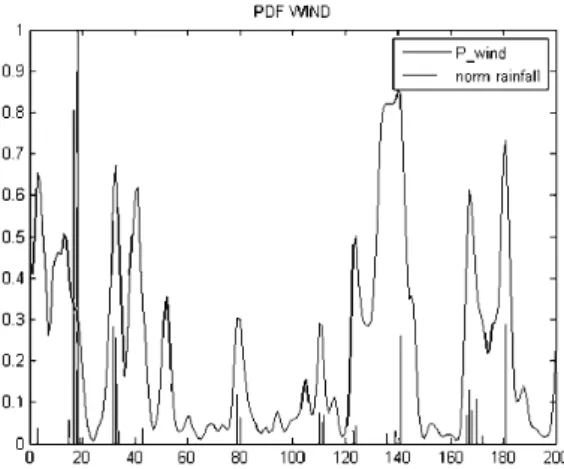
As the geostrophic winds are registered each 12 h, this provides a time series that estimates the rainfall probability. This time series will be named pwin
d-Next figure shows the pwind probability time series for the eary 1999. It can
00 120 140 160 180 200
Fig. 2. Rainfall probability time series pWina with rainfall events
3 Filtering Stage
3.1 Filtering Stage Design
This stage is designed to simplify and extract the useful information from the input data to:
- Obtain simple data where the rainfall information is contained. - Obtain simple series easy to forecast individually.
The idea is, the simpler the time series the easier to forecast. So the input signals are decomposed using the multiscale analysis idea, using a family of convolution filters inspired in the time-scale wavelet concept; see Percibal and Walden (2002), Addison (2002), and Mallat (1999). The family of filters, h(n), is a set of band-pass filters obtained subtracting two gaussian distributions:
h(n) = A exp n2
s + 2 '
N exp
n2 s+l
N
Where A is a scaling coefficient, N is the number of input samples, n is an integer number ( n = 1..N) and S represents the "scale" of the filter. This actually is the rest of two gaussian distributions. The responses of this family of filters in the time domain are represented in left side of Fig. 3 and the right figure shows it in the frequency domain. These have a frequency response similar to the Mexican Hat wavelet, Addison (2002).
•j
r
1 k •-'-. - - - ^
H,W
fff
Fig. 3. Time and frequency response of the multiscale filter
events in time series using filtering stages). Some wavelet transforms, as the Continuous Wavelet Transform (CWT), the Maxima Overlap Wavelet Trans-form (MODWT), the Double Tree Wavelet transTrans-form (DWCWT) preserves also the invariance of the event location among the scales, and consequently, can be used. For example, the Discrete Wavelet Transform (DWT) is not shift invariant.
3.2 Filtering Application: Pe s c, Z500 and Hesc
Three components can be expected in the time series analysis: an stationery periodic component in the low scales/frequencies, the non-stationary components in the middle and high scales/frequencies range. The stationary components of the pressure are well known due to cyclic contributions, and the high frequency scales the main contribution is due to the day/night pressure variations. The middle range variations can be attributed to frontal circulation.
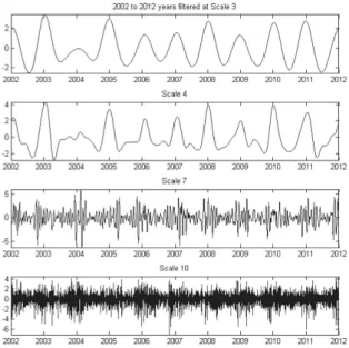
Figure 4 shows the decomposition of the Pesc for scales 3, 4, 7 and 10 through
2002 to the end of 2011. Those signals are obtained filtering Pesc with the Eq. 1.
The filtered signal, at a certain scale, holds the main variations of the signal at a range of time, for instance, scale 2-3 holds the main variations of the signal in one year scale approximately. The signals at scales 10 and above are quite sharp and therefore discarded.
Figure 5 the resulting of filtering Pesc at scales 7, 8 and 9. While in scale 7 the
variation of the signal is to slow to fit the rainfall clusters, at scales 8 and 9 the signal enclose perfectly. The rainfall is bounded by the valleys of the pressure wave. The decomposition of the other time series (Z500 and Hesc) presents a
similar pattern.
In the rest of the article, it is supposed that Pesc, Z500 and Hesc, are the
signals filtered at scale 8 + 9. Note that the selection of the scales is referred to the length of the input vector.
h(n) for N = 4500 samples
1 . 1 1 '. 11 ' 1
2002 to 2012 years filtered at Scale 3
2002 2003 2004 2005 2006 2007 2008 2009 2010 2011 2012 Scale 4
2002 2003 2004 2005 2006 2007 2008 2009 2010 2011 2012 Scale 7
2002 2003 2004 2005 2006 2007 Scale 1C
2009 2010 2011 2012
2002 2003 2004 2005 2006 2007 2010 2011 2012
Fig. 4. Multiscale decomposition of Pesc at low and high scales
4 Classifier Design
The classification stage tries to discriminate if a certain situation corresponds to a rainfall event or not. The selected classifier was a Multilayer Perceptron
(MLP), for its well known classification capabilities.
In the following points there are explained the whole classifier design steps.
4.1 Labelling
The first step is create a features vector to use in the classifier. Actually, this is probably the most important step in the classifier design. In this case, the input data are presented as time series from the initial study (scaled pressure waves, geostropic winds and related variables). As the rainfall events are presented in clusters and usually those clusters are enclosed in the pressure valleys, the feature extraction begins obtaining the time series extremes and performs a set of measurements between one maximum and the following one. The data obtained in a valley without rain, shall be labelled as "Dry" and the data found in a pressure valley with rain shall be labelled as "Rain". This method allows to perform an automatic labelling of the data that simplifies the process (see Shasha and Zhu 2004). Situated in each maximum of Pe s c, there are obtained
Combining Multiscale Filtering and Neural Networks 487
F i g . 5 . Multiscale decomposition of Pesc a t intermediate scales
4.2 F e a t u r e E x t r a c t i o n
To perform the feature extraction, a sequential forward selection (SFS) algo rithm was applied, as it looks for the best training set. It was used a Multilayer Perceptron as selector, Duda (2000). The SFS process tried to classify 100 sam ples with the combinations of 24-features vector. The training results are shown in Fig. 6. The best training set was: [pwind, min PESC, Δ Z5 0 0, Δ He s c] . The error
rises when additional features added, so the process was stopped there.
As a trade off between performance and complexity, the first two features were included in the training vector, since these features need to be forecasted. The other two variables will be included later when the system start to work.
4.3 T e s t V e c t o r s P r e p a r a t i o n
With the selected features, the data needs to be introduced in the Multi Layer Perceptron. The matrix with the input variables is usually called Pmatrix, and
the target vector Tvector. Pmatrix holds [pW I N D, min PESC] sample and Tvector
1 or 0, indicating if the Pdata corresponds to “Rain” and 0 to “Dry”. The dataset
is divided into three subsets: Training dataset, for perform the training of the MLP – (185 vectors). Verification dataset: (185 vectors). Test dataset: Data to test the final classification (300 vectors) (Fig. 6).
488 F.S. Buendia et al.
Fig. 6. SFS process
Fig. 7. MLP hidden layers selection
4.4 Classifier S e t u p a n d T r a i n i n g
Combining Multiscale Filtering and Neural Networks 489
The best performance was achieved with two neurons in the first hidden layer and five in the second, with a classification performance of 87% (25 classification failures in the 185 verification samples). The training was repeated with the network until the number of errors was below 10% of MSE, at the end the network achieved 19 failures in the 185 verification samples, that means a 90% of a priori performance. This value needed to be finally confirmed with the test dataset. 4.5 Classifier performance assessment The network was tested with the test dataset, with vectors not previously used neither to train nor verify the classifier. It appeared 36 failures in 300 samples, that is a 88% of performance. In Table 1 all these data are summarized.
T a b l e 1 . Classification performance summary
Number of samples Number of failures Classification performance
Verification dataset 185
19 90%
Test dataset 300
36 88%
5 Conclusions
This paper presents a complementary method to current forecasts provided by ensembles, as the rainfall is predicted using artificial neural networks and time series. It has been presented the study of the meteorological variables for the local rainfall study, explaining the filtering and classification stages. At the moment, it has been obtained 88% of classification performance that is quite success-ful. Currently, it is being developed the time series forecast, with promissory results. The accuracy and prediction range shall determine the overall system performance. The work continues the presented one in Buendia et al. (2008).
References
Addison, P.S.: The Illustrated Wavelet Transform Handbook, Introductory Theory and Applications in Science, Engineering, Medicine and Finance, 1st edn., 368 p . Taylor & Francis, Abingdon (2002)
Bishop, C.: Neural Networks for Pattern Recognition, 1st edn., 504 p . Oxford University Press, Oxford (1996)
Buendia, F.-S., Tarquis, A.M., Buenda, G., Andina, D.: Feature extraction via multires-olution MODWT analysis in a rainfall forecast system. In: World Multiconference on Systemics, Cybernetics and Informatics 2008 Proceedings, p p . 69–73 (2008) Burton, A., Kilsby, C.G., Fowler, H.J., Cowpertwait, P.S.P., OConnell, P.E.: RainSim:
490 F.S. Buendia et al.
Cowpertwait, P.S.P., OConnell, P.E., Metcalfe, A.V., Mawdsley, J.A.: Stochastic point process modelling of rainfall, I. Single site fitting and validation. J . Hydrol. 1 7 5 , 17–46 (1996)
Dubey, A.D.: Artificial neural network models for rainfall prediction in Pondicherry. Int. J . Comput. Appl. (0975 – 8887) 120(3), 30–35 (2015)
Duda, R.O., Hart, P.E., Stork, D.G.: Pattern Classification, 2nd edn., 680 p . Wiley, New York (2000)
Holton, J.R.: An Introduction To Dynamic Meteorology, 4th edn., 534 p . Academic Press, Cambridge (2004)
Hu, M.J.-C.: Application of the adaline system to weather forecasting. Dissertation Department of Electrical Engineering, Stanford University (1964)
Lorenz, E.N.: The predictability of hydrodynamic flow. Trans. N. Y. Acad. Sci. Ser. II 25(4), 409–432 (1963)
Lorenz, E.N.: Predictability, a problem partially solved. In: Palmer, T., Hagedorn, R. (eds.) Predictability of Weather and Climate, pp. 40–58. Cambridge University Press, Cambridge (2006)
Lovejoy, S., Mandelbrot, B.: Fractal properties of rain, and a fractal model. Tellus A 3 7 A , 209–232 (1985)
Lynch, P.: Chaos, predictability and ensemble forecasting. In: The Emergence of Numerical Weather Prediction: Richardson’s Dream, p p . 229–234. Cambridge Uni versity Press (2006)
Mallat, S.: A Wavelet Tour of Signal Processing, 2nd edn., 620 p . Academic Press, Elsevier, Cambridge (1999)
Percibal, D.B., Walden, A.: Wavelet Methods for Time Series Analysis, 6220 p . Cam bridge University Press, Cambridge (2002)
Rodriguez, M.A.: Predicci´on Meteorol´ogica y Caos en Espacio-Tiempo (Spanish). Revista Espan˜ola de F´ısica 2 2 , 66–69 (2008)
Shasha, D., Zhu, Y.: High Performance Discovery in Time Series, Techniques and Case Studies. Monographs in Computer Science. Springer, Heidelberg (2004)