Aspects of a phased array radar feed and bias network design

(1)

ELE 490 - INDEPENDENT STUDY:

ASPECTS OF A PHASED ARRAY RADAR

FEED AND BIAS NETWORK DESIGN

Electrical Engineering

Date of Defense: 24

th

_{June 2013}

(2)

(3)

PROYECTO FIN DE CARRERA

TEMA: Aspectos de un phased array radar

TÍTULO: Diseño de las redes de alimentación y polarización

AUTOR: Gabriele Galiero Casay

TUTOR: Serhend Arvas

DEPARTAMENTO: L.C. Smith College

CENTRO DE LECTURA: Syracuse University Fecha de Lectura: 24 Junio 2013

Calificación: A

RESUMEN DEL PROYECTO:

(4)

(5)

mientras que los desplazadores de fase necesitarán tensiones continuas que rondan los 10 voltios para proporcionar desplazamientos de fase de hasta 360 grados. En comparación con el sistema de mecánico de rotación, el sistema de polarización diseñado es capaz además de cambiar la directividad de la antena con mayor velocidad. Esto permitirá realizar barridos de 180 grados sin necesidad de mover la antena. Además dichos barridos se pueden realizar a altas velocidades, lo cual supone una ventaja para radares empleados para el seguimiento de objetos en movimiento. Con el objetivo de que dicho sistema sea entendible por cualquier usuario ajeno su diseño, se hace imprescindible la realización de una interfaz gráfica de usuario. Para ello se emplea la herramienta disponible en el entorno de MATLAB, GUIDE, que permite de forma muy intuitiva el desarrollo de interfaces gráficas para usuarios.

Como ya se mencionó anteriormente, se proponen dos soluciones al diseño de la red de polarización de la antena. Cada solución de diseño es sometida a una serie de pruebas mediante la plataforma de MATLAB. Se analizan las ventajas y desventajas de cada una de ellas. Hasta el momento en el desarrollo del sistema de polarización de la antena no ha intervenido la señal de radiofrequencia, empleada para detectar los obstáculos. Dicha señal es generada por una fuente y debe proporcionarse en igual cantidad a cada uno de los ocho elementos del array. Con esta finalidad se diseña una red de alimentación en paralelo, que consiste en el empleo de divisores de potencia de radiofrequencia colocados en paralelo. Esto divide la señal proporcionada por la fuente en partes iguales, y las suministra a los elementos del array. Los divisores de potencia diseñados serán Wilkinsons de 3dB y 0º. Para su diseño se emplea la herramienta AWR2011, que realiza un análisis circuital para la obtención de resultados antes de su fabricación. Esto proporciona una solución aproximada. No obstante se precisaría además de un análisis electromagnético más completo para obtener los resultados de simulación muy próximos a los reales.

Para concluir con el estudio se obtienen una serie de conclusiones acerca de las ventajas que brindan los sistemas de alimentación y polarización diseñados trabajando como parte del sistema de un radar.

(6)

Abstract

Radar technologies have been developed to improve the efficiency when detecting targets. Radar is a system composed by several devices connected and working together. Depending on the type of radar, the improvements are focused on different functionalities of the radar. One of the most important devices composing a radar is the antenna, that sends the radio-frequency signal to the space in order to detect targets. This project is focused on a specific type of radar called phased array radar. This type of radar is characterized by its antenna, which consist on a linear array of radiating elements, in this particular case, eight dipoles working at the frequency band S. The main advantage introduced by the phased array antenna is that using the fundamentals of arrays, the directivity of the antenna can change by shifting the phase of the signal at the input of each radiating element. This can be done using phase shifters. Phase shifter consists on a device which produces a phase shift in the radio-frequency input signal depending on a control DC voltage. Using a phased array antenna allows changing the directivity of the antenna without a mechanical rotating system.

(7)

Resumen

Las tecnologías empleadas por lo dispositivos radar se han ido desarrollando para mejorar su eficiencia y usabilidad. Un radar es un sistema formado por varios subsistemas conectados entre sí. Por lo que dependiendo del tipo de radar las mejoras se centran en los subsistemas correspondientes. Uno de los elementos más importantes de un radar es la antena. Esta se emplea para enviar la señal de radiofrecuencia al espacio y así poder detectar los posibles obstáculos del entorno. Este proyecto se centra en un tipo específico de radar llamado phased array radar. Este tipo de radar se caracteriza por la antena que es un array de antenas, en concreto para este proyecto se trata de un array lineal de ocho dipolos en la banda de frequencia S. El uso de una antena de tipo phased array supone una ventaja importante. Empleando los fundamentos de radiación aplicado a array de antenas se obtiene que la directividad de la antena puede ser modificada. Esto se consigue aplicando distintos desfasajes a la señal de radiofrecuencia que alimenta a cada elemento del array. Para aplicar los desfasajes se emplea un desplazador de fase, este dispositivo aplica una diferencia de fase a su salida con respecto a la señal de entrada dependiendo de una tensión continua de control. Por tanto el empleo de una antena de tipo phased array supone una gran ventaja puesto que no se necesita un sistema de rotación para cambiar la directividad de la antena.

(8)

ACKNOWLEDGMENTS

First and foremost I would like to thank my advisor Mr. Serhend Arvas for his guidance and support that has helped to successfully complete my bachelor’s degree thesis. In addition I would like to thank Mr. Rafael Herradón, subdirector of international relationships of Universidad Politécnica of Madrid, for his continuous advice and allowing me the opportunity of studying abroad to finish my studies in Syracuse University.

(9)

TABLE OF CONTENTS

ELE 490 – ASPECTS OF A PHASED ARRAY RADAR vi

Acknowledgments………..

v

List of figures……….

viii

List of tables………

xi

1. Introduction……….

1

1.1. Definition of Radar……….

1

1.2. Radar parameters………...

3

1.3. Types of Radar………...

5

1.3.1. Frequency band radars………

5

1.3.2. Waveform radars………

5

1.3.3. Tracking radars………

6

1.4. Radar applications……….

7

2. Radar equation………..

9

3. Phased array radar………..

21

4. Feed and bias network………..

25

4.1. Feed network……….

26

4.2. Bias network………..

27

5. Parallel-fed network design………..

28

5.1. Scattering parameters of the 3 dB/0º Wilkinson………

29

5.2. Design and simulation of the 3 dB/0º Wilkinson………

31

5.2.1. Ideal 3 dB/0º Wilkinson……….

32

5.2.2. Real 3 dB/0º Wilkinson………..

34

5.2.3. Real 3 dB/0º Wilkinson at first stage……….

35

5.2.4. Real 3 dB/0º Wilkinson at second stage………..

38

5.2.5. Real 3 dB/0º Wilkinson at third stage………

39

5.3. Parallel-fed network simulation………

41

6. Bias network design………...

45

6.1. Phase shifters………

47

(10)

TABLE OF CONTENTS

ELE 490 – ASPECTS OF A PHASED ARRAY RADAR vii

6.2.1. Function generate_scan………...

49

6.2.2. Function calculate_phaseShift….………

50

6.2.3. Function calculate_phases……….

51

6.2.4. Function toggle……….

52

6.2.5. Function get_voltages………...

55

6.2.6. Function map……….

56

6.3. Arduino Mega 2560 environment and software……….

57

6.3.1. Arduino software…..………..

59

6.3.2. MATLAB Support Package for Arduino……….

62

6.4. Non-inverted amplifiers……….

64

6.5. Graphical User Interface……….

75

7. Conclusion………

77

Appendix A : Fundamentals of electromagnetics………

78

Appendix B : MATLAB functions………

84

Appendix C : Arduino software, test scripts and GUI………...

88

Appendix D : Design Wilkinson details using AWR………..

112

(11)

LIST OF FIGURES

ELE 490 – ASPECTS OF A PHASED ARRAY RADAR viii

LIST OF FIGURES

Fig. 1.1. Scheme of a simple radar using superheterodyne receiver……… 1

Fig. 1.2. Time delay between the transmitted pulse and the received pulse………... 3

Fig. 1.3. Scheme of a radar detecting targets………... 3

Fig. 1.4. Scheme of two different scenarios in detections of multiple targets………. 4

Fig. 1.5. Detection signal used in pulse radars………... 6

Fig. 1.6. Detection signal used in FM-CW radars………... 6

Fig. 2.1. Link of two antennas………... 12

Fig. 2.2. Ideal dipole placed at the origin………... 13

Fig. 2.3. Trigonometric scheme of the ideal dipole radiation……… 14

Fig. 2.4. Equivalent circuit of an ideal dipole receiving signal……….. 17

Fig. 3.1. Different scan angles of a phased array antenna……….. 21

Fig. 3.2. Scheme of a general phased array antenna with infinite elements……… 22

Fig. 4.1. Scheme of a phased array using a parallel feed network………. 25

Fig. 4.2. Scheme of a series-fed array………... 26

Fig. 5.1. Scheme of the parallel-fed array of eight radiating elements……… 28

Fig. 5.2. Microstrip 3dB/0º Wilkinson……… 28

Fig. 5.3. Architecture of the parallel-fed network……… 29

Fig. 5.4. Schematic of an ideal 3dB/0º Wilkinson………. 33

Fig. 5.5. Frequency response of the ideal 3dB/0º Wilkinson……… 33

Fig. 5.6. Substrate defining the parameters of the microstrip line……… 34

Fig. 5.7. Microstrip tee junction………... 35

Fig. 5.8. Resistance with parasitic inductance……… 35

Fig. 5.9. Schematic of a real 3dB/0º Wilkinson……….. 36

Fig. 5.10. Layout of the real 3 dB/0º Wilkinson at the first stage of the feed network……… 36

Fig. 5.11. Frequency response of the real Wilkinson at the first stage……….. 37

(12)

LIST OF FIGURES

ELE 490 – ASPECTS OF A PHASED ARRAY RADAR ix

Fig. 5.13. Frequency response of the real Wilkinson at the second stage……… 39

Fig. 5.14. Layout of the complete feed network……… 40

Fig. 5.15. Frequency response of the real Wilkinson at the third stage……… 40

Fig. 5.16. Schematic of complete parallel-fed network………. 41

Fig. 5.17. Return loss and transmission of the parallel-fed network……… 42

Fig. 5.18. Isolation between some output ports of the parallel-fed network……….. 42

Fig. 5.19. Isolation between some output ports of the parallel-fed network……… 43

Fig. 6.1. Scheme of the bias network……… 45

Fig. 6.2. Software architecture of the bias network……… 46

Fig. 6.3. Phase shift vs. control voltage of the phase shifters……… 47

Fig. 6.4. Points of the phase shift vs. control voltage graph, set by the graph_picker function……….. 48

Fig. 6.5. Generic scan angle of the phased array……… 50

Fig. 6.6. Scheme of the phased array forming a beam……….. 51

Fig. 6.7. Scan angle of 45 degrees and phases of each radiating element………. 54

Fig. 6.8. Scan angle of -45 degrees and phases of each radiating element……… 54

Fig. 6.9. Arduino environment………. 58

Fig. 6.10. Arquitecture of the software using MATLAB Support Package for Arduino…….. 62

Fig. 6.11. Scheme of an operational amplifier………. 64

Fig. 6.12. Equivalent circuit of the ideal operational amplifier……… 65

Fig. 6.13. Virtual short-circuit condition……… 65

Fig. 6.14. Schematic of a non-inverted amplifier……….. 66

Fig. 6.15. Operational amplifier with power supply connections……….. 67

Fig. 6.16. Limitations in a real operational amplifier……….…… 68

Fig. 6.17. Current distribution at the output of the amplifier………... 69

Fig. 6.18. Non-inverted amplifier with small resistance values……….. 70

Fig. 6.19. Non-inverted amplifier with high resistance values……….……… 70

Fig. 6.20. Current source within the real operational amplifier……….. 72

(13)

LIST OF FIGURES

ELE 490 – ASPECTS OF A PHASED ARRAY RADAR x

Fig. 6.22. Scheme of the µA741 operational amplifier with all the terminals………... 73

Fig. 6.23. Schematic of the non-inverted amplifier………... 74

Fig. 6.24. Output vs. input voltage of the non-inverted amplifier……….. 74

(14)

LIST OF TABLES

ELE 490 – ASPECTS OF A PHASED ARRAY RADAR xi

LIST OF TABLES

Table 1.1. Frequency band assignations for radar applications based on ITU. Frequency

band assignations for radar applications based on ITU……… 5

Table 6.1. Parameters of the function generate_scan……… 49

Table 6.2. Parameters of the function calculate_phasesf………. 50

Table 6.3. Parameters of the function calculate_phases………... 52

Table 6.4. Parameters of the function toggle……….. 52

Table 6.5. Cases with different scan angle and phase shift……… 53

Table 6.6. Parameters of the function get_voltages………. 55

Table 6.7. Parameters of the function interp1……… 56

(15)

CHAPTER 1 : INTRODUCTION

ELE 490 - ASPECTS OF A PHASED ARRAY RADAR 1

1. INTRODUCTION

In this chapter a general definition of radar will defined. It will also be shown how it is composed as well as its most important design parameters. Based on the properties of the radar some types of radar will be discussed and finally the most general applications of each type or radar will be mentioned.

1.1. Definition of RADAR

The word radar was originally an acronym, RADAR, for Radio Detection and Ranging. Range in radar communications denotes the distance from the radar to the target.

In general, radars are sensors that send electromagnetic waves into a specific region of space for the detection and location of reflecting objects. The radar sends the electromagnetic waves to the space making use of antennas or antenna systems. When these electromagnetic waves intercept some object (target) within the region they are sent, a portion of the power is reflected and comes back to the radar. These portions of electromagnetic energy are called echoes or radar returns. The receiver has to decide after, amplification of the received signal, if there is or not a target echo.

Once the echoes are identified at the output of the receiver, they are processed to extract target information such as range, velocity, dimension, and other characteristics. In the following figure a scheme of a simple radar is shown.

Figure 1.1. Scheme of a simple radar using superheterodyne receiver.

Each part of the system has different purposes:

(16)

 Generates the signal with the corresponding waveform, depending on the type of radar.

 Modulates the base-band signal, that is going to be used to detect targets, with an RF signal. The base-band signal is modulated because of the propagation characteristics of the waves in the air are better than others, such as waveguides or transmission lines.

 Sets the average power to be transmitted depending on the sensibility of the radar, which means the minimum power that the receiver is able to detect, due to the radar noise. The received power signal must be greater than the sensibility, otherwise the receiver will not detect the echoes.

 Duplexer: Allows bi-directional communication over a single path. It isolates the receiver from the transmitter while permitting them to share a common antenna. It avoids the transmitted signal goes to the detector and breaks it down.

 Antenna: Interface device that allows the electromagnetic waves propagates over the space. By the reciprocity theorem, the behavior of the antenna is the same to receive signal echoes. Then using the parameters of the antenna such as directivity, the transmitter can concentrate the electromagnetic power sent into a specific direction. Also it is possible to change the directivity of the antenna automatically to obtain the target information from several directions.

 RF LNA: A Low-Noise Amplifier is used because of the power of the incoming signal echoes are usually small due to the attenuation of the space, the insertion losses in the objects, diffraction and so on. It has to be low noise level in order to avoid the corruption of the echoes that have low level of power.

 Receiver: It is composed by a detector of the incoming echoes and digital system to process the information of the signal received. The receiver has to decide if the incoming signals are valid echoes or not (clutter) at the output, prior to process the signal to obtain the information. In order to make the decision, the output of the receiver has to be greater than a threshold previously established.

 Detector: It is the most important part of the receiver. In the above figure the detector is a superheterodyne receiver. A superheterodyne receiver demodulates the incoming signal into an intermediate frequency and amplifies it. After that, the obtained signal is demodulated to obtain the band-base signal, that contains the information it is going to be processed.

(17)

 Matched Filter: Is used to improve the signal-noise ratio.

 Display: Eventually, when the receiver determines that the received echo is valid, it proceeds to extract the information in order to display it.

1.2. Radar parameters

Radars have several parameters to detect targets around it and display them in a screen.

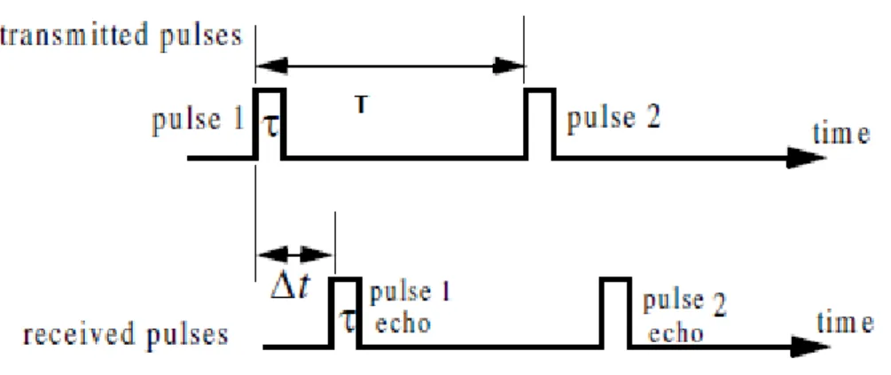
 Range: Range is the distance from the radar to the target. The radar calculates the range, R, from the time delay, of the echoes. The time delay is the time that the signal takes to do a round trip.

Figure 1.2. Time delay between the transmitted pulse and the received pulse.

The range is easily calculated by the following equation:

(1.1)

The factor ⁄ is present because of the signal travels two times the range distance before arriving to the radar.

(18)

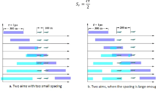
 Range Resolution: It describes the ability of the radar to distinguish between two or more different targets on the same bearing but at different ranges. The range resolution depends mainly on the width of the pulse, , but also depends on the size and distance between targets. A well-designed radar should be able to distinguish targets separated one-half of the pulse width. Then the expression of the range resolution can be written as follows:

(1.2)

Figure 1.4. Scheme of two different scenarios in detection of multiple targets.

In the figure above it can be noted that if the two targets are so close, it can be superposition of echoes (Fig. 1.a). But if the targets are far enough there is no superposition between echoes (Fig. 1.b).

 Doppler Frequency: The Doppler phenomenon consists of a shift in the incident waveform due to the target motion with respect to the source of radiation. The Doppler frequency shift can be written as:

(1.3)

(19)

1.3. Types of Radar

Radars can be classified into several categories depending on its characteristics, such as frequency band, antenna type and waveform used.

1.3.1. Frequency Band Radars

The Institute of Electrical and Electronic Engineers (IEEE), divided the frequency spectrum into several frequency bands. Based on it the International Communications Union (ITU) established specific ranges of frequency within each frequency band which can be used to radar applications.

Frequency Band Nominal Frequency Range Frequency Ranges for radar _{applications based on ITU}

VHF 30-300 MHz 138-144 MHz

UHF 300-1000 MHz 216-225 MHz 420-450 MHz

L 1.0-2.0 GHz 1.215-1.4 GHz 890-942 MHz

S 2.0-4.0 GHz 2.3-2.5 GHz

2.7-3.7 GHz

C 4.0-8.0 GHz 4.2-4.4 GHz

5.25-5.925 GHz

X 8.0-12.0 GHz 8.5-10.68 GHz

Ku 12.0-18.0 GHz 13.4-14.0 GHz

15.7-17.7 GHz

K 18.0-27.0 GHz 24.05-24.25 GHz

24.65-24.75 GHz

Table 1.1. Frequency band assignations for radar applications based on ITU.

1.3.2. Waveform Radars

Radars can be also classified by the waveform used by the transmitter. Based on this classification we can distinguish several types of radars. In this section only some are mentioned.

(20)

Figure 1.5. Detection signal used in pulse radar.

 Pulse compression radar: This type of radar radiates long modulated pulses using frequency or phase modulation. The purpose of using this modulation is to obtain the energy of a long pulse with the resolution of a short pulse.

 Continuous Wave (CW) radar: A sine wave shaped is radiated by the radar. In addition the doppler frequency shift is often used to detect targets in motion.

 _{Frequency Modulation Continuous Wave (FM-CW): A frequency modulation is}

used to allow an improved range measurement.

Figure 1.6. Detection signal used in FM-CW radars.

1.3.3. Tracking Radars

(21)

 Single Target Tracking (STT): Tracks a simple target with enough resolution providing an accurate tracking.

 Automatic Detection and Tracking (ADT): It is able to track several targets. This feature is reached by the measurements of the target locations obtained by several scans of the antenna.

 Phased array tracker: Tracks more than one targets with an electronically scanned phased array. The concept of phased array, that is the topic of this study, it is going to be developed later.

1.4. Radar applications

Depending on the frequency band, there are many radar applications:

 VHF: The first radars were developed to work at this range of frequencies. They were used to military purposes such as detection of ballistic missiles or long range air surveillance. Long range is reached because of the reflection coefficient from earth’s surface is very large at this frequencies, so that the constructive interference of direct signal and the reflected signal from the earth increases the range of detection.

The main inconvenience of this type of radar is the interference with signals generated by other communication systems operating at the same frequencies such as FM and TV broadcast.

 UHF: The main application of this type of radar is long range detection of missiles too. Besides are used to detect and track satellites.

 L band: This band is the most used to long-range air surveillance radars, but the rain could cause problems. That is due to the attenuation of waves at this frequency in presence of the rain. In addition it can be used to detect satellites and ballistic missiles.

 S band: It is used in air surveillance systems for long-range detection, because of measurements are more accurate at this frequency band, although the range is less than VHF and UHF radars. In addition this type of radar is more suitable to obtain a 3D vision of targets. One more application is for near and far weather observation.

 C band: It has similar characteristics and applications as that of S and X band radars.

(22)

 K,Ku band: This frequency band has high range of frequencies, this makes the size of

(23)

CHAPTER 2 : RADAR EQUATION

ELE 490 – ASPECTS OF A PHASED ARRAY RADAR 9

2. RADAR EQUATION

Before defining the radar equation, it is important to recall some definitions of radiation theory. Radiation intensity is the power radiated in a given direction per unit solid angle and can be written as follows:

( ) ( ) ̂ | |

(2.1)

Where the wave is a spherical wave and the expressions of fields are:

⃗ ( ) ⃗ ( ) (2.2)

⃗⃗ ( ) ⃗⃗ ( )

(2.3)

The relationship between them is shown in the following equation:

⃗⃗ ( ) ̂ ⃗ ( ) (2.4)

Where is the intrinsic impedance of the medium.

The total power radiated can be expressed as:

∬ ( ) ⃗⃗⃗⃗ ∬| ( )|

∬

| ( )|

That is equal to the next equation:

∬ ( ) (2.5)

Considering a radar with an isotropic antenna, the power density in the direction of the maximum gain is given by:

(24)

That means the radiation density is constant, the power density is independent on the direction. Therefore the total power radiated by an isotropic antenna is:

∬ ( ) ∬ ∫ ∫

(2.7)

The total power radiated by an isotropic antenna is expressed as follows:

(2.8)

At this point the expression of the power density at a range R can be derived:

| ( )| ( )|

(2.9)

It is known that there are no isotropic antennas in practice. For that reason the gain has to be included in the equation. The directivity of the antenna is defined by:

( ) ( )

( )

(2.10)

The same relationship for a loss-less antenna can be expressed as:

( ) ( ) (2.11)

The gain of the antenna is defined by:

( ) ( )

(2.12)

Where is the power at the antenna input. Generally it is smaller than the radiated power due to the conductor loss. Both the input and radiated power are related by the efficiency:

(2.13)

(25)

Considering an antenna with losses the radiation intensity can be expressed in function of the gain and the radiation intensity of an isotropic antenna:

( ) ( ) (2.14)

The power density at a range R, with a non-isotropic antenna is:

( ) |

( )

( ) (2.15)

When the electromagnetic wave radiated by the radar intercepts with a target, surface currents are induced on it and radiates electromagnetic waves in all directions. The amount of the power radiated is proportional to the target size, material, orientation and shape. All these parameters are integrated in a target parameter called Radar Cross Section (RCS) and is denoted by .

The radar cross section is defined as the ratio of the power reflected back to the radar to the power density incident on the target:

( ) _(2.16)

Where is the power reflected by the target. Therefore the power intercepted by the target is:

( ) ( ) (2.17)

The power travels again a distance R to arrive to the radar and the received power density becomes:

( ) ( ) ( ) ( ) (2.18)

The gain is considered in the direction of maximum radiation:

( ) (2.19)

The equation (2.18) becomes:

(26)

Now to analyze the reception part, all the antennas have a parameter called effective area, which is the ratio of the power available in the antenna receiving signal to the power density of the wave:

| | (2.21)

To determine the relationship between the effective area and gain, it is going to be considered the system showed in the following figure.

Figure 2.1. Link of two antennas.

Suppose two antennas with directivity , and effective area , respectively separated by distance R.

As it was shown before, if the transmitting antenna has a directivity , the power density at a distance R is as the equation (2.15) :

| |

(2.22)

Then the received power by the receiving antenna is:

| |

(2.23)

The same expression can be shown as:

(2.24)

By the reciprocity theorem in electromagnetics it is known that the antennas have the same behavior in both transmitting and receiving. For that reason the transmitting and receiving antenna can be exchanged obtaining the following expression:

(2.25)

(27)

_(2.26)

Once it is known the relationship between directivity and effective area in a link of two antennas we are going to obtain the effective area of a general type of antenna considering a simple case. Suppose that the transmitting antenna is isotropic and the receiving antenna is an ideal dipole:

_(2.27)

The far-fields radiated by an ideal dipole are obtained by calculating the magnetic vector potential and deriving them by Maxwell’s equations. The derivation can be seen in the appendix A (A.3).

Figure 2.2. Ideal dipole placed at the origin.

( ̅)

∭ ( ̅ )

| ̅ ̅ | | ̅ ̅ | (2.28)

As the dipole is ideal, the current density is considered constant along its length:

( ̅ ) ( ) ( ) ̂ _(2.29)

The condition of short (ideal) dipole is given by the following relation:

(28)

Approximations for far-field:

 Amplitude:

| ̅ ̅ | | ̅| (2.31)

 Phase:

| ̅ ̅ | (2.32)

Using trigonometric relations from the triangle formed by the origin, the observation point and the extreme of the ideal dipole, a better approximation can be obtained.

Figure 2.3. Trigonometric scheme of the ideal dipole radiation.

(2.33)

̂ ̂ ̂ ̂ (2.34)

̂ ̂ ̅ ̂ (2.35)

Therefore the distance | ̅ ̅ |_{can be approximated to the following equation:}

| ̅ ̅| ̅ ̂ (2.36)

Using this last approximation the following expression for the phase is obtained:

| ̅ ̅ | ( ) ( ) (2.37)

As | ̅|_and , then . The final approximated expression of the phase can be written as:

| ̅ ̅ | ( ) (2.38) | ̅ ̅ |

(29)

The expression of the magnetic vector potential becomes:

( ̅)

∫ ̂

̂ (2.39)

Then the expressions can be easily derived by the equations described in A.3 (appendix A).

̂ ̂ ̂ ̂ ̂ (2.40)

Where:

( )

(2.41)

( )

(2.42)

We are interested in the electric and magnetic fields, so that to obtain the fields the equations in A.3 (appendix A) have to be used:

⃗⃗ [

( )

] ̂

[ ( ) ] ̂ (2.43)

⃗ ⃗⃗

̂ ̂ (2.44)

Where:

[ ( ) ( ) ] (2.45)

[ ( ) ( ) ] (2.46)

√ (2.47)

Intrinsic impedance of the medium. For free space:

(30)

The expressions of fields contain both the induced and the far-field. Out of all the terms of the equations (2.43) and (2.44), only the far field is considered important. Hence, the near field is neglected. The conditions for far field are the following:

(2.49)

(2.50)

Therefore it can be noted that:

( ) ( ) (2.51)

Taking into account the equation (2.51), the expressions for far field radiated by an ideal dipole can be approximated to:

⃗⃗

̂ (2.52)

⃗

̂ ̂ (2.53)

Hence, the far field wave behaves as a plain wave, although it is a spherical wave.

It is useful to define the radiation pattern as the ratio of the magnitude of the electric field to the maximum magnitude value of the electric field:

( ) ( )

(2.54)

For the case of the ideal dipole the radiation pattern is:

( ) (2.55)

Once the expression of far fields radiated of an ideal dipole, then the next step is to obtain the directivity. As mentioned before in the equation (5.10), directivity is the ratio of the radiation intensity in a certain direction to the radiation intensity of an isotropic antenna.

( )

(31)

Where is the maximum value of the radiation intensity and it is independent on .

( ) | ( )|

| ( )| (2.57)

The radiated power can be expressed as follows:

∬ ( ) ∬| ( )| (2.58)

The directivity expression is simplified to:

∬ ( )

∬| ( )|

(2.59)

Where is called the beam solid angle. For an ideal dipole the beam angle is:

∬| ( )| ∫ ∫

∫

(2.60)

Therefore the directivity of the ideal dipole is:

(2.61)

We recall that all these previous analysis of the ideal dipole has been made to get the effective area of an isotropic antenna. In order to obtain this relation it has only got the effective area of the ideal dipole. This is not intuitive and some more concepts have to be mentioned.

A receiving antenna can be seen as a voltage source transmitting power to a load using a transmission line as a waveguide.

(32)

Where:

Antenna impedance. Antenna resistance. Radiation resistance

Ohmic losses resistance Antenna reactance

Load impedance.

The current of the equivalent circuit can be expressed as:

( ) (2.62)

Taking the magnitude of the current:

| | | |

[( ) ( ) ] ⁄

(2.63)

The receiving power by the load is:

| | | |

( ) ( ) (2.64)

The maximum power transfer theorem establishes that the power transmitted to the load is maximum if:

(2.65)

That establishes:

(2.66)

(2.67)

Considering the case of maximum power transfer, the power received by the load becomes:

| |

(2.65)

(33)

| |

(2.66)

In general the antenna is matched with the transmission line guiding the received wave to the load. That means the antenna impedance is equal to the characteristic impedance of the transmission line.

(2.67)

The maximum power that can be delivered to the load corresponds with the available power at the receiving antenna:

| | | |

(2.68)

Therefore considering the power reflected at the load due to mismatch, the relationship between the power available and the power delivered to the load is:

( | | ) (2.69)

Where is the reflection coefficient at the load:

(2.70)

Matching the load with the transmission line:

(2.71)

After defining the parameter of a receiving antenna, we are going to obtain the effective area of the ideal dipole. First of all we consider that the ideal dipole does not have any losses (

). As it was mentioned before the effective area is:

| |

| | (2.72)

Where:

| | | | _(2.73)

| | | |

(34)

∬| ( )| ∬ ( ) ⃗⃗⃗⃗ (

) ∬ (2.75)

(

) (2.76)

| |

| | (

)

| | (

) ( )

_(2.77)

Then substituting all these terms in the equation of the effective area we obtain:

| |

| | | |

(₎ | |

Once the ideal dipole has been analyzed, the expression of the effective area of an isotropic antenna can be obtained. It is important to remember the expression of the effective area of an arbitrary antenna, obtained considering a link between an isotropic antenna as transmitting antenna and an ideal dipole as receiving antenna.

⁄ (2.78)

If it is considered again a two link antenna with an isotropic antenna as the transmitting antenna ( ) and a general type of antenna as the receiving antenna:

(2.79)

If we consider the efficiency of the antenna then the effective area of a general antenna can be written as follows:

(2.80)

Finally to obtain the received power ( ) by the radar, we have to multiply the effective area of the antenna by the power density incoming given by the equation (2.20):

| |

(35)

CHAPTER 3 : PHASED ARRAY RADAR

ELE 490 – ASPECTS OF A PHASE ARRAY RADAR 21

3. PHASED ARRAY RADAR

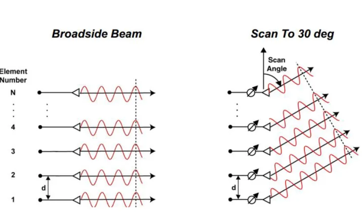
Once the most basic concepts of a radar have been defined, this project is focused on a particular type of radar called phased array radar with eight microstrip dipoles working at a frequency of 2.4 GHz (S band) with a spacing element of ⁄ _{. Phased array radar is characterized by its} antenna. The antenna is a phased linear array of antennas, a set of multiple radiation elements arranged as a straight line, in which the radiation pattern can be reinforced in a particular direction and suppressed in undesired directions. A phased array can provide narrow directive beams that may be steered electronically as shown in the figure 3.1. This is the main advantage of the phase array radar because simply using different phases to the current supplying each array element, the directivity varies. The antenna radar can radiate the electromagnetic power, used to detect targets, in different directions obviating the needed of any mechanical rotation. In addition a phased array can also scan a beam at high electronic speeds and can even have multiple simultaneous main beams.

Figure 3.1. Different scan angles of a phased array antenna.

(36)

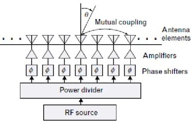
Figure 3.2. Scheme of a general phased array antenna with infinite elements.

The transmitter is compound of a RF source, which generates the radio-frequency signal. After that the power is divided equally to supply each array element with the same amount of power. Phase shifters are responsible for establishing a phase shift in the current supplied to each array element, in order to change the directivity of the antenna. Finally the signal is amplified to be sent and reach targets at long ranges.

An N-element phased array is formed by N identical radiating antennas separated by a distance d along an axis. In the figure above it can be noted that depending on the phase shifts of each element array the interferences of the signal will be constructive in a certain scan angle and destructive in others.

The principle of this type of radar is developed considering the receiver case for simplicity, while similar concepts are held for transmitter case as well due to the reciprocity theorem applied in antennas. Variable time delays are incorporated at each signal path to control the phases of the signals before combining all the signals together at the output. A plain wave-beam is assumed to be incident upon the antenna array at an angle of to the normal direction. Due to the spacing between array elements the beam will experience a time delay in reaching successive antennas, corresponding to the following equation.

(3.1)

Hence if the incident beam is a time-harmonic signal at a frequency f with amplitude of A, the signals received by each of the array elements can be written as:

(37)

The plane wave incident at an angle upon the phased array experiences a linear delay progression at the successive antenna elements. Therefore the variable delay circuits must be set to a similar but with reverse delay progression to compensate for the delay of the signal arrived at the antenna elements. In linear arrays, variable time delays are designed to provide uniform phase progression across the array. Therefore the signal in each channel at the output of the variable delay block can be written as:

_(3.3)

In this equation, denotes the phase difference provided by two successive variable time delay blocks. Therefore the array factor which is equal to the sum of all the signals normalized to the signal at one path can be represented as follows:

∑ ( )

(3.4)

According to equation 3.4, the peak of the array factor occurs at an incident angle which can be determined by:

(3.5)

(

) (3.6)

This angle is called the scan angle. At the scan angle the linear delay progression experienced by the wave arriving at the successive antennas is compensated with the time delays incorporated at each path resulting in constructive interference at the output of the receive array. Therefore the array factor also can be written as the following equation:

[ (

)]

[( )] (3.7)

(38)

of phased array is that the peak gain of the array, according to equation (3.6), can be controlled by electronically tuning the variable time delays eliminating the need for any mechanical system which rotates the antenna array.

(39)

CHAPTER 4 : FEED AND BIAS NETWORK

4. FEED AND BIAS NETWORK OF A PHASED ARRAY RADAR

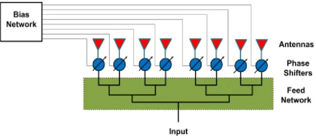
Phased array antennas are usually composed of a feed network and a bias network which allows the operation of the antenna working together. Feed networks are used to distribute the radio-frequency output signal of the transmitter to the radiating elements. There are many ways to feed the arrays. In general array feed networks can be classified into three basic categories: constrained feed, space feed and semi-constrained feed which is a hybrid of the constrained and the space feeds. In a space feed network, the array is usually illuminated by a separate feed horn located at an appropriate distance from the array. Due to the space of the free space between the feed and the radiating elements, this type of feed networks is not a good candidate for planar arrays. This restricts the applications for this type of feed network. The constrained feed, which is usually the simplest method of feeding an array, generally consist of a network which receives the power from an RF source and distributes it to the antenna elements with a feed line and passive elements such as power dividers also known as couplers. The constrain feed itself can be categorized into two basic types: parallel feeds and series feeds. The architectures based on these two feed networks are the most common approach to design phased arrays. The next stage of the phased array is the phase shifters network. Phase shifters can be placed at any stage of phased array. The most common architecture places the phase shifters connecting feed network outputs with each radiating element. Depending on a certain DC control voltage applied to each phase shifter, it produces a certain phase shift at its feed RF signal. Bias network is responsible for controlling automatically these control voltages to form a beam in the desired direction.

Figure 4.1. Scheme of a phased array using a parallel feed network.

(40)

4.1. Feed Network

As mentioned before space feed networks are not suitable for planar arrays, this limits some application for this type of phased array. For the purpose of this project it is going to be considered only constrain feed network, which in turn, is divided into two types: parallel and series feeds.

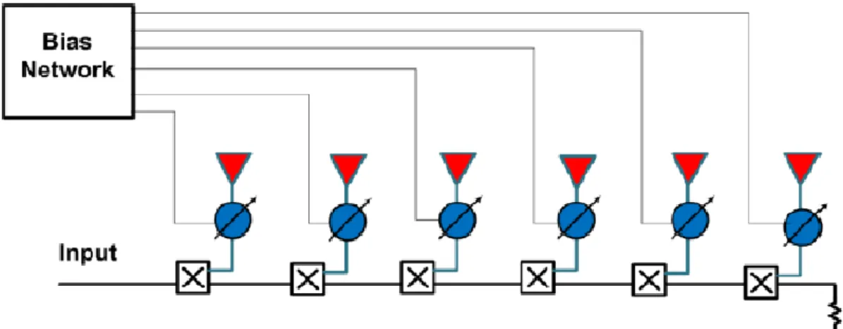
 Series-fed array: In a series-fed array the input signal, fed from one end of the feed network, is coupled serially to the radiating elements of the array as shown in the following figure.

Figure 4.2. Scheme of a series-fed array.

The main advantage of the series-fed array is the compactness. Beside compactness, the small size of the series-fed arrays results in less insertion losses by the feed network. In addition a series-fed array with N elements requires less phase shifters than the parallel-fed arrays. However the cumulative nature of phase shift through the feed network results in an increased beam squint versus frequency, which is one of the main limitations in series-fed designs. The loss through the phase shifters is also cumulative in series-fed arrays which can be an issue in the design of arrays with a large number of array elements.

(41)

Considering the inconveniences given by the series-fed array, a parallel-fed array is chosen for the feed network design developed in the next chapter.

4.2. Bias Network

(42)

CHAPTER 5 : PARALLEL-FED NETWORK DESIGN

5. PARALLEL-FED NETWORK DESIGN

In this chapter the feed network of the array antenna is going to be designed. As mentioned, a parallel-fed array is chosen for this purpose. The array antenna of the phased array radar has eight radiating elements. Therefore using several power dividers the network should provide eight outputs with the same power level, one for each radiating element, from one unique input. The parallel-fed array can be implemented using a tree architecture of power dividers made up of one input port and two output ports as shown in the following figure.

Figure 5.1. Scheme of the parallel-fed array of eight radiating elements.

There are several types of power dividers, but for the specified feed network the 3 dB/0º Wilkinson is the most suitable. This device is a three-port network composed of one input port and two output ports. The power supplied at the input is equally split. The outputs provide half of the input power supplied. The outputs are isolated, and there is no phase shift between them. This type of power divider is often implemented using microstrip lines as depicted in the following figure.

Figure 5.2. Microstrip 3 dB/0º Wilkinson coupler.

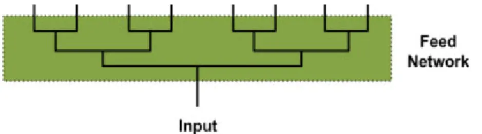
For the parallel-fed network chosen at least seven power dividers are needed. The architecture of the feed network can be divided into three stages. Each stage uses different designs of Wilkinson power divider, as can be seen in the following figure.

Port 1 Port 2

(43)

Figure 5.3. Archiitecture of the parallel-fed network.

The first stage is composed by four power dividers. This results in eight output ports where the dipoles are connected. As it was defined in the chapter 3, the separation between array elements is ⁄ _{. The outputs of the feed network should be separated by a distance of} ⁄ _{. As the design} frequency is 2.4 GHz, the distance between radiating elements is 6.25 cm. Therefore the power dividers at the second and third stage depend on the physical design of the first stage. For this reason, first of all the power dividers of the first stage will be designed. After that, taking into account the element spacing between radiating elements in the array antenna, the power dividers of the second and third stage will be designed. The idea is designing and simulating the power dividers of each stage individually and then simulate the complete feed network. Before designing the power dividers required for the parallel-fed array is important to recall the concept of the scattering parameters of a network. Any radio-frequency device is characterized by its S parameters (Scattering).

5.1. S parameters of the 3 dB/0º Wilkinson

S parameters of a radio-frequency device are defined in function of the incident and reflected power at its ports. The equations for the scattering parameters are the following:

(5.1.1)

(5.1.2)

(5.1.3)

They can also be expressed using matrix form:

[ ] [

] [ ] _(5.1.4)

1st STAGE 2nd STAGE

(44)

Where:

√ (5.1.5)

√ (5.1.6)

Normalized incident power at the port i of the device. Normalized reflected power at the port i of the device.

Incident voltage wave at the port i. Reflected voltage wave at the port i.

The physical meaning of the scattering parameters is the following:

 Reflection coefficient at the port k with the other ports matched:

|

(5.1.7)

 Gain seen at the port k if the port j is stimulated by a generator, with the other ports different from j matched:

|

(5.1.8)

Once the physical meaning of the S parameters has been defined, the next equation shows the S parameters of a 3 dB/0º Wilkinson power divider of the figure 5.2.

√ [

] _(5.1.9)

The behavior of the 3 dB/0º Wilkinson can be deduced by its scattering parameter matrix:

 The reflection coefficient at a given port is zero, when the other ports are matched:

(45)

 The ports 2 and 3 also known as the output ports are isolated:

(5.1.11)

 The power at the output ports of the device is one-half of the input power. The output signal of each port are in phase:

√ (5.1.12)

The factor j reflects the phase difference between the input and output signal, due to the line of length ⁄ which results in an electrical length of 90 degrees.

If the incident power and reflected power at a general port i are defined as follows:

| | (5.1.13)

| | (5.1.14)

Therefore the scattering parameter can be obtained from the equation (5.1.2) as:

|

(5.1.15)

Taking the magnitude the following relationship can be obtained:

| |

| | | |

(5.1.16)

The ratio of the reflected power at the port two to the incident power at the port one is one half. The result is obtained between the third port and the first one as establish equation (5.1.12).

5.2. Design and simulation of a 3 dB/0º Wilkinson using AWR

In this section it is going to be designed the above described power divider using the radio frequency software AWRDE 10. Before designing the power divider it is important to define some design characteristics such as the operation frequency and the substrate used:

 Design frequency: (S band).  Substrate characteristics:

(46)

 Dielectric thickness:  Conductor thickness:  Loss tangent:

 Electrical resistance:

This parameter is the electrical resistance of the conductor normalized with respect to the electrical resistance of the gold. The electrical resistance at 20-25 degrees Celsius is:

(5.2.1)

_(5.2.2)

Therefore the value of RHO is obtained from the following equation:

(5.2.3)

Once the basic design characteristics are defined, the design can be started. First of all the ideal case is simulated. It consists of using ideal transmission lines, loss-less, to implement the tracks and ports of the power divider. This gives a first approach of the final design solution. After that in order to obtain a more accurate design, real transmission lines can be used in the design. These real transmission lines are lossy lines whose characteristic parameters are defined by its substrate. Therefore, in order to finish the analysis, the physical schematic is obtained and the circuit is implemented. Finally some measures are taken to ensure the well operation of the power divider.

5.2.1. Ideal 3 dB/0º Wilkinson

As mentioned before, the ideal simulation consists on a first approach solution design using loss-less transmission lines. It only produces a phase difference. The schematic of the power divider is shown in the figure 5.4.

The characteristic impedance of the ports and line transmissions used is 50 Ω. The values of the characteristic impedance of the tracks and resistance match with the values from the figure 5.2.

(47)

Figure 5.4. Schematic of an ideal 3 dB/0º Wilkinson.

Figure 5.5. Frequency response of the ideal 3 dB/0º Wilkinson.

RES ID=R1 R=100 Ohm

TLIN ID=TL2 Z0=70.71 Ohm EL=90 Deg F0=2.4 GHz TLIN

ID=TL1 Z0=70.71 Ohm EL=90 Deg F0=2.4 GHz

PORT P=3 Z=50 Ohm PORT P=2 Z=50 Ohm

PORT P=1 Z=50 Ohm

2 2.2 2.4 2.6 2.8

Frequency (GHz)

Frequency Response Ideal Wilkinson

-70 -60 -50 -40 -30 -20 -10 0

2.4 GHz

-3.01 dB DB(|S(1,1)|)Ideal Wilkinson

DB(|S(2,1)|) Ideal Wilkinson DB(|S(3,1)|) Ideal Wilkinson

DB(|S(2,2)|) Ideal Wilkinson

(48)

The figure above shows the different values of the scattering parameters in dB at different frequencies. As it can be noted at the operation frequency:

( ) ( ) | | | | (5.2.1.1)

Therefore:

(5.2.1.2)

Also the relation between the input and output ports can be seen in the following scattering parameters in dB:

( ) | | (5.2.1.3)

( ) | | (5.2.1.4)

Therefore:

| | | | (5.2.1.5)

This means that the power at the output ports is one-half of the power at the input port as it is desired. The isolation between the output ports can be seen analyzing the parameter or , which are close to minus infinite.

5.2.2. Simulation of a real 3 dB/0º Wilkinson

Once a first approach has been obtained, the next step is to simulate the 3 dB/0º Wilkinson using microstrip lines. In order to obtain accurate results the substrate used has to be completely characterized. Using AWRDE 10 software, the substrate can be characterized using the element in the following figure:

Figure 5.6. Substrate defining the parameters of the microstrip line.

(49)

After defining the substrate it is used to implement the power divider, the lines have to be defined. Microstrip lines have two design parameters: physical length and width. These two parameters are set by the tool TXLine that calculates the physical length and the width of each line using several input parameters such as frequency, type of conductor, impedance, electrical length, dielectric constant and so on. These values match whit those of the figure 5.2. The conductor of the substrate used is copper.

As there are lines with different width, there will be some parasitic effects. These effects should be taken into account using the element MTEE shown in the following figure.

Figure 5.7. Microstrip tee junction.

Another effect to take into account is the parasitic inductance present at the resistance even using SMD components. This effect it can be included in the simulation using the element in the following figure.

Figure 5.8. Resistance with parasitic inductance.

The schematic of the real 3 dB/0º Wilkinson is shown in the figure 5.9. This schematic it is going to be used for all the following power divider designs. Each design will have different values of physical length and width of the lines.

5.2.3. Simulation of a real 3 dB/0º Wilkinson at the first stage

The output ports of the power divider should have a distance between them equal to ⁄ . This occurs because the array elements should be separated by half-wavelength. It is important to design the power dividers considering the layout from the beginning. The first stage is composed by four power dividers. In the figure 5.10 is shown the layout of the real Wilkinson at the first stage.

1 2

3 MTEE

ID=TL23 W1=1.441 mm W2=1.441 mm W3=2.782 mm

(50)

Figure 5.9. Schematic of a real 3 dB/0º Wilkinson.

Figure 5.10. Layout of the real 3 dB/0º Wilkinson at the first stage of the feed network.

1 2 3 MTEE ID=TL12 W1=1.441 mm W2=1.441 mm W3=2.782 mm 1 2 3 MTEE ID=TL11 W1=1.441 mm W2=1.441 mm W3=2.782 mm SRL ID=RL1 R=100 Ohm L=0.5 nH PORT P=2 Z=50 Ohm MLIN ID=TL17 W=1.441 mm L=4.5 mm MLIN ID=TL24 W=2.782 mm L=5 mm MLIN ID=TL22 W=1.441 mm L=5.7 mm PORT P=1 Z=50 Ohm MLIN ID=TL18 W=1.441 mm

L=4.5 mm PORTP=3

(51)

The schematic used for the above layout is the same as the figure 5.9. Once the length and the width of the lines are set by the tool TXLine, the schematic is simulated to obtain the scattering parameters. Using the Tune tool the length of the lines can be modified to optimize the frequency response of the device.

Figure 5.11. Frequency response of the real Wilkinson at the first stage.

As noted in the figure above, the value of the scattering parameters are as desired. The output ports provide half of the input power. The output ports can be considered isolated between them:

( ) | | (5.2.3.1)

This can be expressed in linear scale as follows:

| |

(5.2.3.2)

Therefore it can be considered a good approach. Also the reflection coefficient is almost zero. Then the first stage of the design of power dividers it can be considered as a good solution.

2 2.2 2.4 2.6 2.8

Frequency (GHz)

Frequency Response Real Wilkinson 1st Stage

-60 -50 -40 -30 -20 -10 0

2.4 GHz -3.259 dB

2.4 GHz -36.36 dB

2.4 GHz -38.12 dB

2.4 GHz -44.08 dB

DB(|S(1,1)|) Real Wilkinson

(52)

5.2.4. Simulation of a real 3 dB/0º Wilkinson at the second

stage

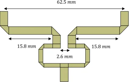
The second stage of the feed network is composed by two power dividers. The layout needed is shown in the figure 5.12.

The length addition of the output lines of the second stage Wilkinson of the feed network is not exactly half of the distance between outputs, because it has to be considered the space where the resistance is connected. More other details have to be considered such as the width of the lines. Therefore, the schematic of the Wilkinson couplers in the second stage of the feed network is the same as the first stage, but changing the values of the lines at the output ports. Although the length of the output ports is modified, the frequency response should be the same as the first stage power dividers.

Figure 5.12. Layout of the second and first stage of the feed network.

The frequency response of the Wilkinson power dividers at the second stage is shown in the figure 5.13.

(53)

Figure 5.13. Frequency response of the real Wilkinson at the second stage.

The power reflected by the power divider is very small. In addition the output ports can be considered isolated between them because of the small value of the scattering parameter . Finally, the output ports provide approximately half of the input power.

5.2.5. Simulation of a real 3 dB/0º Wilkinson at the third

stage

The third stage of the feed network is composed by only one power divider. The layout considering all the stages is shown in the figure 5.14.

The schematic of the Wilkinson coupler in the third stage of the feed network is the same as the first stage, but changing the values of the lines at the output ports. The length of the output ports are shown in the figure 5.14. After setting the length of the output lines, the power divider has to be simulated individually. The frequency response obtained in simulation is shown in the figure 5.15. The results obtained are similar to the frequency response of the power dividers at the first and second stage. Therefore the real 3 dB/0º Wilkinson at the third stage works as desired.

2 2.2 2.4 2.6 2.8

Frequency (GHz)

Frequency Response Real Wilkinson 2nd Stage

-60 -50 -40 -30 -20 -10 0

2.4 GHz -3.39 dB

2.4 GHz -36.31 dB

2.4 GHz -38.38 dB

2.4 GHz -43 dB

DB(|S(1,1)|) Real Wilkinson 2

(54)

Figure 5.14. Layout of the complete feed network.

Figure 5.15. Frequency response of the real Wilkinson at the third stage.

2 2.2 2.4 2.6 2.8

Frequency (GHz)

Frequency Response Real Wilkinson 3rd Stage

-60 -50 -40 -30 -20 -10 0

2.4 GHz -3.65 dB

2.4 GHz -36.82 dB

2.4 GHz

-38.9 dB 2.4 GHz -41.37 dB

DB(|S(1,1)|) Real Wilkinson 3 DB(|S(2,2)|) Real Wilkinson 3 DB(|S(2,1)|) Real Wilkinson 3 DB(|S(3,1)|) Real Wilkinson 3 DB(|S(3,2)|) Real Wilkinson 3

(55)

5.3. Parallel-fed network simulation

Once the Wilkinson power dividers of each stage have been simulated and optimized individually, they should be connected forming the parallel-fed network shown in the following figure.

Figure 5.16. Schematic of the parallel-fed network.

The simulation will reflect the operation of each stage of the feed network. The above schematic consists of a ten-port network. This results in a large number of scattering parameters. The most important are which describe the return losses, transmission and the isolation between output ports. The frequency response is shown in the following figures.

PORT P=6 Z=50 Ohm PORT P=5 Z=50 Ohm PORT P=4 Z=50 Ohm PORT P=3 Z=50 Ohm PORT P=2 Z=50 Ohm PORT P=1 Z=50 Ohm 1 2 3 SUBCKT ID=S6

NET="Real Wilkinson 2"

1

2 3

SUBCKT ID=S4

1

2 3

SUBCKT ID=S3

1

2 3

SUBCKT ID=S2

1

2 3

SUBCKT ID=S7

1

2 3

SUBCKT ID=S5

1

2 3

SUBCKT ID=S1

(56)

Figure 5.17. Return loss and transmission of the parallel-fed network.

Figure 5.18. Isolation between some output ports of the parallel-fed network.

2 2.2 2.4 2.6 2.8

Frequency (GHz)

Frequency Response Parallel Fed Network 1

-60 -50 -40 -30 -20 -10 2.4 GHz -46.41 dB 2.4 GHz -10.3 dB DB(|S(1,1)|) Feed Network DB(|S(2,1)|) Feed Network DB(|S(3,1)|) Feed Network DB(|S(4,1)|) Feed Network DB(|S(5,1)|) Feed Network DB(|S(6,1)|) Feed Network DB(|S(7,1)|) Feed Network DB(|S(8,1)|) Feed Network DB(|S(9,1)|) Feed Network

2 2.2 2.4 2.6 2.8

Frequency (GHz)

(57)

Figure 5.19. Isolation between some output ports of the parallel-fed network.

As noted the return losses of the feed network are:

( ) | | (5.3.1)

In the linear scale of values this is approximately zero:

| |

(5.3.2)

In addition the transmission characteristics of the network can be seen by the following scattering parameters:

( ) ( ) ( ) (5.3.3)

In the linear scale this is approximately: