Mixed Integer Quadratic Programming based predictive control for hydrogen production using renewable energy

Texto completo

(1)PREPRINT. Mixed-Integer-Quadratic-Programming based Predictive Control for Hydrogen Production Using Renewable Energy Alvaro Serna Dept. de Ingeniería de Sistemas y Automática. University of Valladolid (UVA). Valladolid, Spain. [email protected]. Fernando Tadeo Dept. de Ingeniería de Sistemas y Automática. University of Valladolid (UVA). Valladolid, Spain. [email protected]. Abstract— An Energy Management System (EMS) to. balance the production of renewable sources with the consumption by a set of electrolization units is proposed here based on Model Predictive Control ideas (MPC). This EMS regulates the operating point of each electrolyzer and its connections or disconnections using a Mixed-Integer-Quadratic-Programming algorithm. A case study is given for an installation composed of wave and wind energy sources and a set of 3 alkaline electrolyzers. Validation using measured data at the target location of the installation shows the adequate performance of the proposed EMS. Keywords—hydrogen; renewable energy; predictive control. I.. INTRODUCTION. Hydrogen might offer great advantages over traditional energy carriers [1], as long as it is produced from renewable energy sources [2]. Different renewable energy sources have already been studied for electrolyzation, such as wind [3], waves [4] and solar energy [5,6]; the feasibility of these sources to produce hydrogen has been demonstrated, with the main drawback their variability [6, 7]. Hybrid sources have been proposed to partially overcome this variability [8]. Electrolyzation is a mature, market-available technique that can operate intermittently, producing large volumes of hydrogen, without greenhouse gases emissions, if electricity is provided by renewable sources. There exist several promising electrolysis technologies [2], such as polymer electrolysis (PEMEC), alkaline cells and solid oxide electrolysis (SOEC) [9]. All of them are capable to generate hydrogen with a purity better than 99.97%, which is the quality used in the automotive industry [10]. The This work was funded by Ministerio de Ciencia e InnovaciónDPI2014-54530-R. H2Ocean received funding from the European Union Seventh Framework Programme (FP7/2007-2013) under grant agreement nº 288145.. Julio E. Normey-Rico Dept. de Automação e Sistemas. Universidade Federal de Santa Catarina (UFSC). Florianópolis, Brazil. [email protected]. electrolyzers considered here are Alkaline Electrolyzers as they are available at the required power levels (about MW) to make the technology cost-efficient for this application (see [7,11] for details). In the proposed Energy Management System, power consumption adapts to the available power by connecting or disconnecting electrolyzation units and regulating the operating points of the ones that are connected, thus following a smart grid approach for the local microgrid [2]. Compared with previous proposals [2,4], this paper concentrates on using an advanced control system to maximize the production and reduce the number of connection/disconnections (in order to improve the state of health of the electrolyzers). The proposed EMS is based on Model Predictive Control ideas. Model predictive control (MPC) is popular in industry since the 1990s and there is a steadily increasing attention from control practitioners and theoreticians [12]. The proposed approach makes possible for system operators to know in advance the expected production and, therefore, schedule preventive-predictive maintenance operations on the electrolyzer units. For simplicity, in this work the produced energy is fully used (no storage or external sources are considered), but the results can be easily extended to the most common situation of using only the excess of energy from renewable sources [7,13]. A preliminary version of this proposal was presented in [8] and it is fully developed and refined here. Moreover, a non-linear model with discrete and continuous variables is proposed here which is then modified into a MIQP (MixedInteger Quadratic Programming). The rest paper is organized as follows: Section II presents the installation and summarizes MPC ideas. The proposed EMS is presented in Section III. Section IV presents the case study used and its validation using measured data from the target location. Some conclusions are presented at the end of the paper..

(2) PROCESS DESCRIPTION. Fig. 1 presents the components of the proposed sustainable hydrogen plant [8]. Renewable energy sources (wind and wave) provide energy to the process. The EMS has as objective to adapt the production of hydrogen to the available power using the degrees of freedom of the control system in such way that production is maximized without degrading the electrolyzation units.. point for the two types of electrolyzers that will be presented in the case studies of Section 4. 600 Hi (Nm3H2/h). II.. High Production Electrolyzers Small Production Electrolyzers. 400 200 0. Renewable Energy Sources. % Operating point (α) Figure 2. Hydrogen production of the electrolyzers.. Demineralized Water (H2O). Electricity Hydrogen (H2). Electrolysis Figure 1. General scheme of the electrolysis plant.. A. Manipulated variables  The manipulated variables are the operating points for each electrolyzer. They are defined by αi (k) where: a). It is 0 if the electrolyzer is disconnected.. b) Takes values inside [ αi α ̅i ] if it is connected, αi > 0 and α ̅i < 1.  In addition, binary variables δi (k) ϵ {0,1} are used, where 0 corresponds to electrolyzer disconnection and 1 to electrolyzer connection.. C. Model Predictive Control The main advantage of MPC is the fact that it takes explicitly into account performance specifications and constraints [14]. The main elements in MPC are depicted in Fig. 3 [12]: the optimization block receives information from the model block which is responsible for computing the predictions of the output of the plant in a defined horizon. This model uses the current and past measured process outputs and inputs in order to update the predictions at each sample time along a prediction horizon named N. In the optimization block, a set of constraints are considered as well as the future references for the process outputs. Cost Function Constraints. Future References. +. u Optimization. -. Sequence of Future Controls. Electrolyzer models are represented by the following equations: ̂i (k) ̂ i (k)∙δ α ̂ i (k)+b a∙α. ⋅ ̅ Pi. Control. Output Model. B. Model and controled variables. ̂ i (k) = H. Plant. Predicted Outputs Figure 3. Model Predictive Control scheme..  MPC uses a receding horizon strategy, thus, although a set. of future control moves are computed in the optimization   block, only the first control action of the sequence is applied and the procedure is repeated at the next sampling time [12]. ̂ ̂ where equations Pi (k) and Hi (k) are the controlled ̂i (k) is the predicted power III. PROPOSED ENERGY MANAGEMENT SYSTEM variables of electrolyzer i: P consumption of each device at time k and ̅ Pi is its maximum ̂ i (k) is the predicted hydrogen production at power, while H As it was mentioned in Section 1, alkaline electrolyzers ̅i are used to define were selected. Different alkaline electrolyzers are assumed the same sample. Parameters ai , bi and P the device performance, that is, the relationship between in this paper being n the number of devices the suffix and i consumed power and production. Note that electrolyzer is used to identify each device. In the rest of the paper, k models are static, because the time required for the devices represents the discrete time in samples (a sample time of 1 to change the operation point from min to max power is less hour is typically used). than 5 minutes in the worst case, therefore, these dynamics can be neglected as the usual sampling time for the Energy Management System is 1 hour. Fig. 2 depicts the hydrogen production of the electrolyzers as a function of the operating ̂i (k) = ̅ P Pi ∙ α ̂i (k) ∙ δ̂i (k).

(3) A. Control objectives The MPC proposed aims to maximize the hydrogen production taking into account the limitation in the available power and the operational constraints. The three objectives can be defined as: O1 To maximize the hydrogen production, the difference between the value of the prediction for each electrolyzer production and its maximum value is minimized for all the electrolyzers along the prediction horizon. O2 To maximize the operation of the electrolyzers, the binary variables which defines the ON-OFF condition must be, when possible, equal to 1 (ON condition) along the prediction horizon. O3 Power consumed by the set of electrolyzers must be always smaller than the power provided from the renewable energies but will try to be equal. B. Cost function and optimization problem The following quadratic cost function, solved each sample time, is considered in the optimization problem: 2 ̂ ̅ J = ∑ni=1 ∑N j=1[(Hi (k + j) − Hi (k + j)) Q Hi N. u ̂ ̂ (k + j − 1))2 Q ] + ∑ni=1 ∑j=1 (δi (k + j) − δ i δi. Here, we transform problem (4) into a mixed-integer quadratic problem with linear constraints (MIQP). To do it, first each electrolyzer model is modified using the following change of variable: zi (k) ≐ αi (k) ∙ δi (k)   where zi ∈ ℝ. The hydrogen production model is now:. (3). Thus, using equation (3), all the system constraints and the electrolyzer models, the optimization problem to be solved at each sample time is (4). (4). ̂ i (k) = H. ẑi (k) a∙ẑi (k)+b. As it can be seen, because of the non-linear model of the electrolyzer and the use of binary and real decision variables, the MPC problem to be solved by the algorithm is. . ̅i ⋅ P. Hi (zi (k) + Δzi (k + 1)) = Hi (zi (k)) +. ∂Hi ∂zi. ∙ Δzi (k + 1). . Therefore, simplifying the notation and applying the same procedure for the N predictions of the hydrogen production, gives: bi ̂ i (k + 1) ̂ i (k+1) = Hi (k) + H ∙ Δz (a ∙z (k)+b )2 i. i. i. bi ̂ i (k + 1)+ Δz ̂ i (k + 2)) ̂ i (k+2) = Hi (k) + H ∙ (Δz (a ∙z (k)+b )2. ̂ i (k+N) = Hi (k) + H. i. i. ⋯ bi (ai ∙zi (k)+bi )2. ⋯ ̂ i (k + 1) + Δz ̂ i (k + 2) + ∙ (Δz. ̂ i (k + Nu )) ⋯ Δz. ̅i ⋅ P. ̂i (k) ≤ P ̂available (k) ∑ni=1 P. . Hi is now a real function of the real variable zi, and as zi is in the [0,1] interval, a > 0 and b > 0, Hi (zi) is continuous and differentiable in the interval [0,1]. Despite the change made in equation (8), this equation is not linear in variable z yet and it must be approximated. If H is not linear in z, the relationship between H (k+j) and z (k+j) will not be linear either. It is necessary to make another approximation in the predictions to change the problem into a MIQP. To linearize future predictions of the hydrogen production, an approximation has been done using a first order truncation Taylor series:. ⋯. ̂i (k) = P ̅i ∙ α P ̂i (k) ∙ δ̂i (k). . As a static model is considered, the predictions of the produced hydrogen do not depend on past values. In equation (6) it can be seen that H = 0 when δ = 0, so it can be rewritten as (8) to remove the dependence between Hi and αi:. i. αi ≤ αi ≤ α ̅i. . ̅i ⋅ P. ̂ i (k)+b a∙α. ̂i (k) = P ̅i ∙ ẑi (k)  P. δ ∈ [0, 1]. ̂i (k) ̂ i (k)∙δ α ̂ i (k)+b a∙α. ẑi (k). ̂ i (k) = H. ̂ i (k) ≐ H. To solve this problem, the future predictions of the hydrogen production are expressed as a function of the future control actions and the past values of the input and outputs using the electrolyzers model (1) and (2).. st:. C. Approximation to a MIQP. . which takes into account, in a prediction and control horizons of N and Nu samples respectively, the error ̂ i ) and its between the predictions of produced hydrogen (H ̅ i ) and also penalizes the number of desired values (H connections and disconnections. Moreover, Q Hi and Q δi are the weighting factors for the error and control action respectively. The first term of (3) is used for objective O1 of section 3.1 while the second term of this equation tries to achieve objective O2.. Min J (αi , δi ). a NLMIQP (Non-Linear Mixed Integer Quadratic Problem) which is very difficult to solve. Thus, in the next section a simple solution is proposed.. Defining gi ≐. bi (ai ∙zi (k)+bi )2. . , vector 1 ≐ [1 1 … 1]T (dimension. 1xN) and matrix T∈ℝNxNu is:.

(4) Nu 1 1 𝐓≐ 1 1 [1. 0 ⋯ ⋯ 1 0 ⋯ 1 1 0 N 1 1 1 1 1 1]. . ̂𝐢 ̂ 𝐢 = 1∙ Hi(k) + gi ∙T∙ 𝚫𝐳 𝐇.  . where: ̂ 𝐢 ≐ [Δz ̂ i (k+1) ……Δz ̂ i (k+Nu)]T 𝚫𝐳. . The manipulated variables are Δzi (k), αi (k) and δi (k). Therefore, the relationship between prediction and manipulated variables can be written using the vector of future control movements which is given by (15): Δzi (k + 1) Δzi (k + 2) ⋯ Δzi (k + Nu). 𝚫𝐮𝐢 ≐. 𝚫𝐳𝐢 αi (k + 1) αi (k + 1) = 𝛂𝐢 ⋯ αi (k + Nu) [ 𝛅𝐢 ]. . . Hi = fi + Gi ∙ 𝚫𝐮𝐢. (17). Thus:. In (17) fi is the free response, computed using the nonlinear model (8) for Hi(k) and Gi. 𝚫𝐮𝐢 is the linealized forced response [12,15]. Considering now the set of n electrolyzers:. where:. N. . u zi (k) + ∑l=1 Δzi (k + l)≥ αi ∙δi (k+Nu). u zi (k)+ ∑l=1 Δzi (k + l) ≤ αi (k + 1) − αi (1-δi (k+Nu)) . N. . αi (k) ≤ α ̅i. . αi (k) ≥ αi. . In addition to the constraints before, the following constraint is considered to fulfill the objective O3: The total power consumed at each sample (k) should be smaller than the predicted power available from the renewable energies ̂available (k)). Taking into account model predictive control (P ideas, the vector of predictions of available power, ̂available (k), is calculated over the prediction horizon using P meteorological data. Thus, the constraint in the consumed powers is:. As can be seen, all the defined constraints in equations (2329) are linear in the decision variables Δz, α and δ. This allows to solve the problem as a MIQP. E. Optimization. The MPC problem of minimizing the cost function (4) subject to (23-29) can be transformed into a quadratic Mixed-Integer Quadratic Programming (MIQP):  𝟏 𝐓 𝐓 Min (𝟐 𝚫𝐔 ∙ 𝐌 ∙ 𝚫𝐔 + 𝐥 ∙ 𝚫𝐔)  𝚫𝐔 s.t 𝐀 ∙ 𝚫𝐔 ≤ 𝐁  . where H and f are a N∙nx1 vectors and ΔU is a Nu∙nx1 vector, follows: H = f + G∙ΔU. . ̂i (k) ∙ ẑi (k) ≤ P ̂available (k) k = 1, 2, .., N  ∑ni=1 P. Gi = [gi∙T 0 0]. ΔU ≐ [ΔU1 ΔU2 … ΔUn]T. N. u zi (k) + ∑l=1 Δzi (k + l)≤ α ̅i ∙δi (k+Nu). N. where 𝚫𝐮𝐢 ∈ ℝ3Nu. Gi ∈ ℝ Nx3Nu is:. f ≐ [f1 f2 … fn]T. As it was said in the previous section, a new variable z was added to solve the problem. The constraints were changed into a MLD (Mixed Logical System, [16,17]) to associate the behavior of the plant with the continuous variable α and the binary variable δ and to linearize them. The following constraints (23-28) show this idea for all the cases where the binary variable could be 0 or 1:. u zi (k)+ ∑l=1 Δzi (k + l) ≥ αi (k + 1) − α ̅i (1-δi (k+Nu)). δi (k + 1) δi (k + 2) ⋯ [ δi (k + Nu) ]. H ≐ [H1 H2 … Hn]T. . D. Constraints. The vector of predictions for each i is given by: ̂ i ≐ [H ̂ i (k+1) ……H ̂ i (k+N)]T H. 𝐆𝟏 0 0 0 0 𝐆𝟐 0 0 G≐ [ ] 0 0 ⋯ 0 0 0 0 𝐆𝐧. . to be solved at each sample time (𝐀 and B are the constraints matrices of the problem). Using equation (3) in the original cost function gives:.

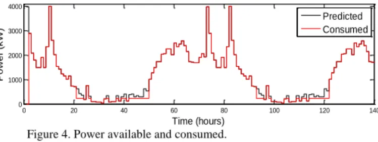
(5) ̅ )𝐓 𝐐𝐇 (𝐟̂ + 𝐆 𝚫𝐔 − 𝐇 ̅) 𝐉 = [(𝐟̂ + 𝐆 𝚫𝐔 − 𝐇.  H = [485. . ̂ − 𝟏) 𝐐𝛅 (𝛅 ̂ − 𝟏)] +(𝛅 𝐓. α = [1 1 1]T. ̂ , and And considering the relationship between 𝚫𝐔 and 𝛅 manipulating (31) gives the cost function to be minimized: 𝟏. 𝐉 ≐ 𝟐 𝚫𝐔 𝐓 ∙ 𝐌 ∙ 𝚫𝐔 + 𝐥𝐓 ∙ 𝚫𝐔. 485 50]T. QH. = [1. α = [0.2 0.2 0.1]T. 1 50]T. Q δ = [1 1 1]T. . Some results for 140 hours of operation are shown in Fig. 48. The results confirm the correct operation of the advanced Matrices 𝐌, 𝐥 are the quadratic and the linear part of the control system for the parameters considered in this case quadratic problem respectively and are given by: study. Fig. 4 shows the power provided by the renewable energy sources (black line) and the consumed power (red 𝐌 ≐ [𝐆𝐓 𝐐𝐇 𝐆 + 𝐐𝛅 ]   line). As can be appreciated in the simulations, the controller tries to maintain the consumed power very near 𝐓 𝐓 𝐓 ̅ 𝐥 ≐ [𝟐𝐟 𝐐𝐇 𝐆 − 𝟐𝐇 𝐐𝐇 𝐆 + 𝟐(𝟏 𝐐𝛅 )]  the available one and as consequence obtaining a hydrogen production near the achievable maximum. In this case, consumed power could have a maximum Finally the constraints (23-29) can be written in the compact form 𝐀 ∙ 𝚫𝐔 ≤ 𝐁. Note that the dimensions of the matrices value of 4488 kW (2134 kW for each high production depend on the prediction and control horizons (N and Nu) electrolyzer and 220 kW for the small production electrolyzer) if all the electrolyzers worked at a 100%. and the number of electrolyzers (n). IV. CASE STUDY A. Components The sources considered in this case study are wind and wave: wind energy as it is a mature technology [18] and wave energy as it provides lower variability in the energy production [19]. One vertical axis wind turbine (VAWT) of 5.0 MW peak power and one wave energy converter (WEC) of 1.6 MW peak power were selected accordingly to the studies developed in the H2Ocean* project [20]. To produce hydrogen, different NEL A485 electrolyzers (NELHydrogen, 2014) were chosen.. Power (kW). 4000. Predicted Consumed. 3000. 2000. 1000. 0. 0. 20. 40. 60. 80. 100. 120. Figure 4. Power available and consumed.. Fig. 5 shows the performance of the electrolyzer i = 1 (maximum power: 485 Nm3/h). As expected, it is not switched on/off very frequently and the operating point is always between α and α.  (i=1)  (i=1). 1. B. EMS implementation of the electrolysis An MIQP solver in the Matlab® CPLEX was used to carry out the optimization in (23). To validate the EMS a sampling time of one hour was used. In this proposal the current available power at each time k is different for the one predicted in the previous step. The values of αi and αi were defined using data from the electrolyzer manufactures. C. Results and discussion of the case study To validate the proposed EMS, meteorological data in a specific location in the Atlantic Ocean was used. A simulation was developed using three electrolyzers (two high production and one small production), thus n=3. A prediction horizon of three hours and a control horizon of one hour where chosen. Thus N=3 and Nu=1. The parameters of the platform are: P = [2134. 2134 220]T. 0 0. a = [0.875 0.875 0.778. b = [3.525 3.525 3.625]T. 20. 40. 60. 80. 100. 120. 140. Time (hours). Figure 5. Operation of electrolyzer 1.. Fig. 6 shows the operation of the second electrolyzer i = 2 that also produces an amount of 485 Nm3/h. As in the case before, the values of α are between the minimum and maximum bounds.  (i=2)  (i=2). 1. 0 0. ]T. 140. Time (hours). 20. 40. 60. 80. Time (hours). Figure 6. Performance of electrolyzer 2.. 100. 120. 140.

(6) Electrolyzer i = 3 (Fig. 7) is more connected because its performance is better than the other electrolyzers, so the operation of this electrolyzer can be considered correct. In all cases, the values are between the minimum and maximum values that were defined.  (i=3)  (i=3). 1. 0 0. 20. 40. 60. 80. 100. 120. [3]. Andrews, J. and Shabani, B. Re-envisioning the role of hydrogen in a sustainable energy economy, International journal of hydrogen energy, 37 (2), pp. 1184-1203. 2012.. [4]. Serna, A., Torrijos, D., Tadeo, F. and Touati, K. Evaluation of wave energy for a near-the-coast offshore desalination plant. In World Congress on Desalination and Water Reuse (IDA) 20-25 October 2013 Tianjin, China. pp. 1-7. [5]. Martínez, M., Molina, M.G., Machado, I.R., Mercado, P.E. and Watanabe, E.H. Modelling and simulation of wave energy hyperbaric converter (WEHC) for applications in distributed generation, International Journal of Hydrogen Energy, 37 (19), pp. 14945-14950. 2012.. [6]. Joshi, A.S., Dincer, I. and Reddy, B.V. Solar energy production: A comparative performance assesstement, International Journal of Hydrogen Energy, 36 (17), pp. 11246-11257. 2011.. [7]. Floch, P.H., Gabriel, S., Mansilla, C. and Werkoff, F. On the production of hydrogen via alkaline electrolysis during off-peak periods, International Journal of Hydrogen Energy, 32 (18), pp. 46414647. 2007.. [8]. Serna, A., Normey-Rico, J.E. and Tadeo, F., Model predictive control of hydrogen production by renewable energy. In International Renewable Energy Congress (IREC), 2015 6th International IEEE. pp. 1-6.. [9]. Ebbesen, S.D., Jensen, S.H., Hauch, A. and Mogensen M.B. High Temperature Electrolysis in Alkaline Cells, Solid Proton Conducting Cells, and Solid Oxide Cells, Chemical Reviews, 2014.. 140. Time (hours). Figure 7. Performance of electrolyzer 3.. Finally, Fig. 8 depicts the evolution of the total hydrogen production by the three electrolyzers in this case study: Hydrogen (Nm3/h). 1000 800 600 400 200 0. 0. 20. 40. 60. 80. 100. 120. 140. Time (hours). Figure 8. Hydrogen production by the electrolyzers.. V.. CONCLUSIONS. A solution to the energy management of an electrolyzation plant powered by variable renewable energy sources has been presented and evaluated. Using Smart Grid ideas, a model predictive control strategy has been proposed, where the characteristics of each electrolyzer is taken into account to maximize the production and improve the state-of-health of the units. Validation using data measured from the target location is carried out to show the correct operation of the plant with the developed controller. ACKNOWLEDGMENT This work was also funded by Ministerio de Ciencia e Innovación DPI 2014-54530-R Most of this work was carried out during a stage of A. Serna at the research group of Prof. Normey-Rico in Florianópolis (Brazil). We thank Karsten Agersted (DTU, Denmark) for his generous contribution to his work. Prof. Normey-Rico thanks CNPqBrazil for financial support. REFERENCES [1]. [2]. Balable, A. and Kotb, H. Analysis of a hybrid renewable energy stand-alone unit for simultaneously producing hydrogen and fresh water from sea water, International Journal of Thermal and Environmental Engineering, 6 (2), pp. 55-60. 2013. Serna, A. and Tadeo, F. Offshore hydrogen production from wave energy, International Journal of Hydrogen Energy, 39 (3), pp. 15491557. 2014.. [10] Petersen, H.N. Note on the targeted hydrogen quality produced from electrolyser units, Review of the Department of Energy Conversion and Storage, Technical University of Denmark, 2012. [11] Ganley, J.C. High temperature and pressure alkaline electrolysis, International Journal of Hydrogen Energy, 34 (9), pp. 3604-3611. 2009. [12] Camacho, E.F. and Bordons, C. Model predictive control, Springer, 2013. [13] Gutiérrez-Martín, F., Confente, D. and Guerra, I. Management of variable electricity loads in wind–hydrogen systems: the case of a Spanish wind farm. International Journal of Hydrogen Energy, 35 (14), pp. 7329-7336. 2010. [14] Khalid, M. and Savkin, A.V. A model predictive control approach to the problem of wind power smoothing with controlled battery storage, Renewable Energy 35 (7), pp. 1520-1526. 2010. [15] Plucenio, A., Pagano, D.J., Bruciapaglia, A.H., Normey-Rico, J.E. A practical approach to predictive control for nonlinear processes. In: NOLCOS 2007, 2007. Proceedings of the NOLCOS 2007, 2007. [16] Bemporad, A., Morari, M. Control of systems integrating logic, dynamics, and constraints. Automatica, 35(3), 407-427. 1999. [17] da Costa Mendes, P.R., Normey-Rico, J.E., Bordons, C. Economic Energy Management of a Microgrid Including Electric Vehicles. Innovative Smart Grid Technologies Conference Latinoamerica (ISGTL 2015, Montevideo, Uruguay). [18] Dietrich, K., Latorre, J.M., Olmos, L. and Ramos, A. Demand response in an isolated system with high wind integration. Power Systems, IEEE Transactions on, 27 (1), pp. 20-29. 2012. [19] Stoutenburg, E.D., Jenkins, N. and Jacobson, M.Z. Power output variations of co-located offshore wind turbines and wave energy converters in California, Renewable Energy, 35 (12), pp. 2781-2791. 2010. [20] H2ocean-project.eu,. 'H2ocean'. N.p., 2015. Web. 23 Sept. 2015. Available at http://www.h2ocean-project.eu/..

(7)