New methods for the estimation of Takagi-Sugeno model based extended Kalman filter and its applications to optimal control for nonlinear systems

New methods for the estimation of Takagi-Sugeno model based

extended Kalman filter and its applications to optimal control

for nonlinear systems

Basil M. Al-Hadithi*'^, Agustín Jiménez and Fernando Matía

Intelligent Control Group, Universidad Politécnica de Madrid, Madrid, Spain

SUMMARY

This paper describes new approaches to improve the local and global approximation (matching) and model-ing capability of Takagi-Sugeno (T-S) fuzzy model. The main aim is obtainmodel-ing high function approximation accuracy and fast convergence. The main problem encountered is that T-S identification method cannot be applied when the membership functions are overlapped by pairs. This restricts the application of the T-S method because this type of membership function has been widely used during the last 2 decades in the stability, controller design of fuzzy systems and is popular in industrial control applications. The approach developed here can be considered as a generalized versión of T-S identification method with optimized per-formance in approximating nonlinear functions. We propose a noniterative method through weighting of parameters approach and an iterative algorithm by applying the extended Kalman filter, based on the same idea of parameters' weighting. We show that the Kalman filter is an effective tool in the identification of T-S fuzzy model. A fuzzy controller based linear quadratic regulator is proposed in order to show the effective-ness of the estimation method developed here in control applications. An illustrative example of an inverted pendulum is chosen to evalúate the robustness and remarkable performance of the proposed method locally and globally in comparison with the original T-S model. Simulation results indicate the potential, simplicity and generality of the algorithm. An illustrative example is chosen to evalúate the robustness. In this paper, we prove that these algorithms converge very fast, thereby making them very practical to use. Copyright ©2011 John Wiley & Sons, Ltd.

KEYWORDS: nonlinear systems; fuzzy systems; Takagi-Sugeno fuzzy model; extended Kalman filter; linear quadratic regulator

1. INTRODUCTION

Nonlinear control systems based on the Takagi-Sugeno (T-S) fuzzy model [1] have attracted lots of attention during the last 20 years (e.g., see [2-7]. It provides a powerful solution for the development of function approximation, systematic techniques to stability analysis and controller design of fuzzy control systems in view of a fruitful conventional control theory and techniques. They also allow relatively easy application of powerful learning techniques for their identification from data. This model is formed by using a set of fuzzy rules to represent a nonlinear system as a set of local affine models which are connected by fuzzy membership functions. This fuzzy modeling method presents an alternative technique to represent complex nonlinear systems [8] and reduces the number of rules in modeling higher order nonlinear systems [1] and [2],

Some papers focus on the proof of the universal approximation property of the T-S fuzzy models as they are able to approximate any smooth nonlinear functions to any degree of accuracy in any *Correspondence to: Basil M. Al-Hadithi, Intelligent Control Group, Universidad Politécnica de Madrid, José Gutiérrez

convex compact región [9], [4], [10], and [8]. But it was clearly shown by several researchers that the number of fuzzy rules increases as the approximation error tends to zero [11]. This exponential growing cannot be eliminated, so it becomes difficult to make use of the universal approximation property of the T-S fuzzy modeling for practical purposes. In addition to that, it was shown in [12] that the set of functions, consisting of polytopic or the T-S models constructed from finite number of rules, is nowhere dense in the approximation model space, if that is defined as a subset of contin-uous functions. As a consequence, by means of the mentioned models, it is difficult to approximate in general, continuous functions arbitrarily well if the number of rules are restricted. Thus, only the functions satisfying certain conditions can be approximated by such models, or alternatively, an unbounded number of rules are required. This result is considered as a limitation for such models. The solution suggested by the authors for this discrepancy can be the trade-off between the accuracy and the number of rules.

These conflicting objectives have motivated the researchers to find a balance between the specified accuracy and the computational complexity of the resulting fuzzy model.

Recently, a great interest has been shown to Tensor Product Distributed Compensation (TPDC) as an established controller design framework that links the TP model transformation and parallel distributed compensation framework. The TP model transformation converts different models to a common representational form [13]. In [14], the approximation capabilities of the TP model forms are analyzed, because the universal applicability of the TPDC framework strongly relies on it. It has been shown that the practically important subset of the TP model forms that uses bounded number of rules has limited approximation capability: the set of such TP model forms lie nowhere dense in the space of continuous functions. Such cases require the use of trade-off techniques between accuracy and the TP model forms complexity. It has been shown that the uniform applicability of the TPDC framework is guaranteed, because the TPDC enables the use of trade-off methods. This is a great advantage of over analytic transformation, where such considerations are hardly possible to apply

The definition of higher order singular-value-decomposition (HOSVD) canonical form was firstly proposed in [15]. The authors introduced how the concept of tensor HOSVD can be carried over to the TP dynamic models, namely, how the 'HOSVD like' decomposition of linear parameter varying dynamic models can be defined and generated. The authors ñame this decomposition as HOSVD based canonical form of the TP model or polytopic model form. The key idea and the basic concept of this decomposition was proposed recently with the TP model transformation based control design methodology. The novelty of this work is to present the mathematical background of this concept. The paper shows convergency theorems how the TP model transformation is capable of recon-structing this HOSVD based canonical form numerically. The proofs of the theorems are lengthly, therefore they are omitted. The paper also presents numerical examples to show the applicability, efficiency, and uniformity of the numerical reconstruction.

In [16], the HOSVD based canonical form of linear parameter varying models [15] is analyzed and a models's most important invariant characteristics is shown. The numerical reconstructibility of the HOSVD canonical form using the TP model transformation is studied. Convergency theorems for given numerical reconstruction constraint are presented.

In [17], a singular value-based method for reducing a given fuzzy rule set was discussed. The method conducís singular valué decomposition of the rule consequents and generates certain linear combinations of the original membership functions to form new ones for the reduced set. The work characterizes membership functions by the conditions of sum normalization, non-negativeness, and normality. The proposed method is applicable regardless of the adopted inference paradigms. The present work discusses three specific applications of fuzzy reduction: fuzzy rule base with singleton support, fuzzy rule base with nonsingleton support, and the T-S model.

Great attention has been paid to the identification of the T-S fuzzy models and several results have been obtained [19], [9], and [20]. They are based upon two kinds of approaches, one is to linearize the original nonlinear system in various operating points when the model of the system is known, and the other is based on the input-output data collected from the original nonlinear system when its model is unknown. The authors in [19] use a fuzzy clustering method to identify the T-S fuzzy models, including identification of the number of fuzzy rules and parameters of fuzzy mem-bership functions and identification of parameters of local linear models by using a least squares method [21]. The goal is to minimize the error between the T-S fuzzy models and the corresponding original nonlinear systems.

In [22], Klawonn et al. explained how fuzzy clustering techniques could be applied to design a fuzzy controller (FC) from the training data. In [23], Hong and Lee have analyzed that the disadvan-tages of most fuzzy systems are that the membership functions and fuzzy rules should be predefined to map numerical data into linguistic terms and to make fuzzy reasoning work. They suggested a method based on the fuzzy clustering technique and the decisión tables to derive membership functions and fuzzy rules from numerical data. However, Hong and Lee's algorithm presented in [23] needs to predefine the membership functions of the input linguistic variables and it simplifies fuzzy rules by a series of merge operations. As the number of variables becomes larger, the decisión table will grow tremendously and the process of the rule simplification based on the decisión tables becomes more complicated. The authors in [9] suggest a method to identify the T-S fuzzy models. Their method aims at improving the local and global approximation of the T-S model. However, this complicates the approximation in order to obtain both targets. It has been shown that constrained and regularized identification methods may improve interpretability of constituent local models as local linearizations, and locally weighted least squares method may explicitly address the trade-off between the local and global accuracy of the T-S fuzzy models.

In [21], a new method of interval fuzzy model identification was developed. The method com-bines a fuzzy identification methodology with some ideas from linear programming theory. The idea is then extended to modeling the optimal lower and upper bound functions that define the band which contains all the measurement valúes. The method can be efficiently used in the case of the approximation of the nonlinear functions family.

In [24], a new approach to fuzzy modeling using the relevance vector learning mechanism (RVM) based on a kernel-based Bayesian estimation is introduced. The main concern is to find the best struc-ture of the T-S fuzzy model for modeling nonlinear dynamic systems with measurement error. The number of rules and the parameter valúes of membership functions can be found as optimizing the marginal likelihood of the RVM in the proposed Fuzzy Inference System (FIS). Because the RVM is not necessary to satisfy Mercer's condition, selection of kernel function is beyond the limit of the positive definite continuous symmetric function of Support Vector Machine (SVM). The relaxed condition of kernel function can satisfy various types of membership functions in fuzzy model.

In [25], the authors suggest a transformation method that offers a trade-off between the modeling complexity and accuracy of the T-S fuzzy model. The suggested transformation method is aimed at finding the minimal number of fuzzy rules for a given accuracy of a given T-S fuzzy model. Opti-mization of the approximation trade-off is conceptually obtained by the discarding of those rules, which have weak or no contribution at all to the output.

Interpolation is an important subject for reducing dense rule bases as well for deriving useful information from sparse ones. In [11], the authors show that rule interpolation helps in reducing the identification complexity as it allows rule bases with gaps. It is suggested that only the minimal necessary number of rules remain which contain the essential information, and all other rules are replaced by the interpolation algorithm.

The approach proposed in [11] has some drawbacks such as subnormal conclusión for certain configuration of the involved fuzzy sets and does not always lead to interpretable fuzzy membership functions. In [26], a new technique for fuzzy rule interpolation was investigated. The aim is to com-bine the advantageous computational behavior of [11] and at the same time reduces the disadvantage of subnormality.

deficiencies, for instance, it does not always result in immediately interpretable fuzzy member-ship functions. In [27], an approach is presented to get rid of these disadvantages. It is based on the interpolation of relations instead of interpolating a-cut distances and which offers a way to derive a family of interpolation methods capable of eliminating some typical deficiencies of fuzzy rule interpolation techniques.

In [28], a generalized versión of the previous Cartesian approach [29] for interpolating fuzzy rules of membership functions with finite number of characteristic points is presented. Instead of repre-senting membership functions as points in Cartesian spaces, they now become elements in the space of square, integrable function. Interpolation is thus made between the antecedent and consequent function spaces. The generalized representation allows an extended class of membership functions satisfying two monotonicity conditions to be accommodated in the interpolation process.

In [1], the authors develop an interesting method to identify nonlinear systems using input-output data. They divide the identification process in three steps; premise variables, membership func-tions, and consequent parameters. With respect to the membership funcfunc-tions, they apply nonlinear programming technique using the complex method for the minimization of the performance index.

In [30], a study has outlined a new min-max approach to the fuzzy clustering, estimation, and identification with uncertain data. The proposed approach minimizes the worst-case effect of data uncertainties and modeling errors on estimation performance without making any statistical assumption and requiring a priori knowledge of uncertainties.

Several methods are used to deal with the problem of optimizing membership functions, which are either derivative-based or derivative-free methods. The derivative free approaches are desirable because they are more robust than derivative-based methods with respect to finding global minimum and with respect to a wide range of objective function and Membership Functions (MFs) types. The main drawback is that they converge more slowly than derivative-based techniques [31].

On the other hand, derivative-based methods tend to converge to local minimums. In addition, they are limited to specific objective functions and types of inference and MFs. The most com-mon approaches are: gradient descent [32], least squares [21], back propagation [33], and Kalman filtering [34], [35].

Kalman filter, is a powerful mathematical tool for stochastic estimation from noisy environment. It has various applications in optimizing fuzzy systems. For example, it has been used to extract fuzzy rules from a given rule base [36] and to optimize the output function parameters of the T-S fuzzy systems. Fuzzy logic has been used to compute the gains of a bank of parallel Kalman filters in order to combine their outputs [37]. The fuzzy logic has also been used to tune the parameters of the Kalman filter [38].

The use of the Kalman filter training to optimize the MFs of a fuzzy system was introduced by Simón [34] for motor winding current estimation. The used MFs were assumed as symmetric trian-gular forms. The Kalman filter training was extended to asymmetric triangles in [35], and a matrix was defined relating the parameters of the MFs together based on the sum-normality conditions, then projecting this matrix in each iteration of optimization to constrain the MFs to sum normal types.

Because the derivatives of the functions are used in Kalman filtering, it is limited to special type of MFs because of complicated and time consuming calculations. So far only triangular types are optimized for both inputs and outputs of an Fuzzy Logic Controller (FLC) [34,35].

As we will demónstrate in this article, the T-S model cannot be applied when the member-ship functions are overlapped by pairs. The methods presented here are characterized by the high accuracy obtained in approximating nonlinear systems locally and globally in comparison with the original T-S model.

2. ESTIMATION OF THE FUZZY T-S MODEL'S PARAMETERS

An interesting method of Identification is presented in [1]. The idea is based on estimating the non-linear system parameters minimizing a quadratic performance index. The method is based on the identification of functions of the following form:

f-.m"

_m

y = f(xu x2,..., x„)

Each IF-THEN rule Rll-ln, for an nth order system can be written as follows:

S(h...in) . l í X i i s Mh a n d _Xn i s Min m e n

y = ^''1-''»> + p^-in)Xl + p^-ín)X2 + ... _Fnn(.h—in) _xr _n

where the fuzzy estimation of the output is:

£íí=i---££=i«>

'

-

'"

(*)

* 2 _M ( í ' l - í ' n ) .

£2

"-££=i«>

'

-

'"

00

(i)

(2)

where,

w (í'l-í'n) (x) = / ¿ i¿ 1 (Xi)ll2i2 (X2) . . . \Lnin (Xn) being [ijij (XJ), the membership function that corresponds to the fuzzy set M '.

Let M be a set of input/output system samples {x\k,x2k,•••,x„k,yu}- The parameters of the

fuzzy system can be calculated as a result of minimizing a quadratic performance index:

J = Y,<yk-yk)

= \\Y-xp\

where

Y =

P =

y

. yi

'

-pí

1

B1 -_ Hm

yi ••• ym

•1) ^ d . . . ! ) , ( 1

••» tf~»x

1 fí(1"1}x,

Hm Al m •

Y

-

... pi

-• -• -• P l -XTII

• •Hm xnm

•1) _ ( r i - r n ) • • Po

o(r\-rn)

o(r\-rn)

Hm

•.P^1

•P[n -oín.

• Hm -rn)

xn\

•rn)Y

and

(3)

(4)

3 (í'l-í'n) W (í'l-í'n) fot)

ní

---£^=i'«

'

-

'"

(^)

If X is a matrix of full rank, the solution is obtained as follows:

/ Y - XP ||2 = (Y - XP)T(Y - XP)

P = (XTXylXTY

V / = XT(Y - XP) = XTY - XTXP = 0

(5)

3. RESTRICTIONS OF THE T-S IDENTIFICATION METHOD

The method proposed in [1] arises serious problems as it cannot be applied in the most common case where the membership functions are those shown in Figure 1.

The membership functions ftifc) = ,' I*' and «.¿2te) = l' Z"J are defined in an interval [ÜÍ, bi] which should verify:

IMi(ai) = \ [in(bi)=0 IM2(ai) = 0 i-ii2(bi) = 1

IM\(xi) + iHiixi) = 1

For this case which is widely used, it can be easily demonstrated [39] that the matrix X is not of full rank and therefore XT X is not invertible, which makes the mentioned method of T-S invalid.

This result can be easily proven as follows: Supposing that it exists:

/ : mn — • SR

y = m

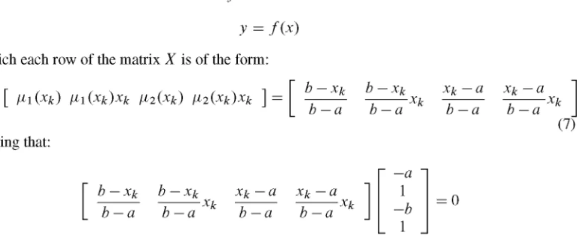
in which each row of the matrix X is of the form:

Xk = [ Mi te) Miteü-x/t M2te) ¡ii{xk)xk 1 = - — í * - — ^X k

L o —a o — a verifying that:

Xk Xk

~Xk

(7)

xk xk xk

Xk

-r-xk-a

•a -xk

1

The rank of X in this case is 3. In other words, the columns of X are linearly dependent which in turn makes impossible the use of the aforementioned identification method proposed in [1], Analyzing another example of two variables:

f : W m

y = f(xl,x2)

Each row of the matrix X is of the form:

Xk = [/¿n/^21 t^\\t^2\X\k HllH2lX2k MllM22 t^\\t^22X\k ^11^22^2*

/¿12M21 t^\2t^2\X\k t^\2t^2\X2k M12M22 t^\2t^22X\k Ml2M22^2/t] (8) It can be noticed that the columns 1, 3, 4, and 6 have the same form as in the previous example multiplied by a constant ¡i\\ and therefore, they are linearly dependent as well. The same thing happens with the columns 6, 9, 10,12, and so on. In fact, the rank of the matrix in this case is 8.

1

V-a Ha

The solution proposed in [1] avoids the occurrence of this situation. In order to identify a function in the interval [a¡, b¡] using the T-S method, certain intermedíate points are chosen of the form:

a* e [ai,bi] andb* e [úf¿,¿¿] and they use membership functions which verify:

(9)

0 a¡ ^ x ^ a*

t¿i2(x) = { xi-a* * ^ ^ , (10) -¿—|r a* ^ x ^ bi

b¡ -a¡ i

and thus:

liil(ai) = l íiil(b*) = 0

IMi(a*) = 0 iii2(bi) = 1

which impedes that the domains of these functions being overlapped and therefore it can be observed that, except for some isolated points,

IM\(xi) + IHiixi) ^ 1

and thus, in general, the matrix X will be of full rank and the method is applicable. This solution can be clearly seen in [1] where the authors find the optimum membership functions minimizing the performance index and reducing the problem to a nonlinear programming one. For this reason, they use the well-known complex method for the minimization. This can obviously be observed in the illustrative examples selected by the authors in [1] where all the identified memberships are nonoverlapping ones.

4. NONITERATIVE APPROACH

The restriction of the T-S identification method for the case presented in the previous section does not mean the nonexistence of solutions rather than an incentive for their search. As it has been seen, the problem comes from the fact that the solution should fulfil:

VJ = X'Y -X'XP = 0 (11) But as it was shown earlier, the columns of the matrix X are linearly dependent and consequently

X'X is not an invertible matrix, therefore it is impossible to calcúlate P through:

P = (X'xy^X'Y (12) Nevertheless, as the rows of X' are linearly dependent, the independent term in (11) X'Y will

have the same dependence among its rows and thereupon, the rank of the system matrix will be the same as the rank of the extended matrix with the independent term.

rank (X'X) = rank(X'X\X'Y)

And so, the system has a solution. In other words, the system is a compatible indeterminate one, that is, if P is a solution of (11) and K belongs to the Kernel of X'X,

KeKeriX'X)

4.1. Parameters' weighting method

An effective approach with few computational effort, based on the well known parameters' weight-ing method, is proposed. The main target is to improve the choice of the performance index and minimize it. It is characterized by extending the objective function by including a weighting y of the norm of P vector.

J

= J2(yk-nf

+ Y

J2P!

= w

~

w

+ y

w

w

This can be rewritten as foliows:

/ = \\Y -XPf + y , ..2 \\p\\2 Y 0

X

\Ya-XaP\

Now, the extended matrix Xa is of full rank, and the vector P can be computed as:

P = (XaXa) XaYa

(13)

(14)

(15)

Obviously, the solution that minimizes this index is not optimum. However, for a small valué of y , it will be cióse to the optimum one and it will be unique as well.

The weighting of y does not need to have a unique valué, rather than some valúes can be weighted more than others to choose the most suitable one.

/

= E^-^)

E^i

i i

-

i i

ii

i

fe=i

Y 0

X

r

where T is a diagonal matrix formed by the valúes y2 which should necessarliy have a valué other than zero to guarantee that the extended matrix is invertible.

4.2. Parameters tuning using the parameters' weighting method

The parameters' weighting method can also be used for parameters tuning of the T-S model from local parameters obtained through the identification of a system in an operating región or from any physical input/output data.

We suppose that in this case, we have a first estimation

M) - LPo P\ ?2 • • • Pn\

of the T-S model parameters. In order to obtain such an estimation, the classical least square method can be used around the equilibrium point. The objective is to obtain a global approximation of the system.

y P°o ¿>i*i P2X2 Pnxn

Let us analyze a setof input/output system sampleslx^.^/t,... ,x„k,yk}- The parameters of the global approximation can be calculated by minimizing the following quadratic performance index:

where

/ =

Y

Po

xs

= £(*

= [*

= U°

" i i

i

-h)2= \\Y-XgP0\\2

yi P°r xu

x12

X\m

ys ••• ym \

P°2 ••• P°n]T

Xi\ . . . Xn\ X22 • • • X„2

X2m • •• Xnm

(17)

In this case, if we select a sufficient number of points distributed in the región where it is required to obtain the approximation, then the matrix Xg will be of a full rank and therefore, the solution

becomes unique, which can be calculated as follows:

Po — (X Xg) X Y (19)

This first approximation can be utilized as reference parameters for all the subsystems. Then, the parameters' vector of the fuzzy model can be obtained minimizing:

rn n

k = \ ¿1 = 1 ¿«=i j=o 2

0 (¿l-¿n)\2 _\Y-Xp\\

2 + y2\\p0-p\

Y

ypo

x

where

\Ya~Xap\

po = [P0P0... Po?

(20)

r\.r2—rn

In this case, the factor y represents the degree of confidence of the parameters initially estimated. In a similar way to the previous case, different weight factors of yj1-'"' can be used to each one of

the parameters py~ln> depending on the reliability of the initial parameter p°j in the specific rule. rn n

J = I > - h)

+J2---J2H y?

-

»

üv° - Pj

"^)

fc=l

Y

r>

¿ 1 = 1 ¿„ = l j = 0 2

\Ya-Xap\

\r(p0-p)\\'

(21)

,(¿l-¿«)

where T is a diagonal matrix with the weight factor v " . It is not necessary to apply this process for all the parameters. If the valúes of some of them are known, they can be fixed beforehand or we

(¿i-¿«)

can assign them a weighting factor yj "; comparatively high.

5. ITERATIVE PARAMETERS' IDENTIFICATION

The inconvenient feature of the aforementioned method is the amplification of the matrix X through-out the time, so that it becomes inappropriate to be used in real time applications as adaptive control for example. The solution is find an iterative method so that the dimensión of the calculation will not be augmented for each sample. As explained in detail in Section 3 that the solution developed in [1] to find the optimum membership functions is invalid when memberships are overlapping ones. In this section, we use an iterative method based on the extended Kalman filter to solve with this problem.

5.1. The Kalman filter

The Kalman filter is widely used for stochastic estimation. It is developed by Rudolph E. Kalman, through a recursive method for the discrete data linear filtering [40]. The Kalman filter is known to be optimum for linear systems with white process and measurement noises. It is assumed that the system is described by the foliowing sampled model:

x(k + 1) = $x(k) + Tu{k) + v(k)

y(k) = Cx(k)+e(k) (22)

where x (k) represents the state of the dynamic system, u (k) is the input vector and y (k) is the output vector. The vector v(k) represents the Gaussian-white noise of the system and e(k) is the measured Gaussian-white noise. Both of them are independent from each other with zero mean. The objective of the Kalman filter is to obtain an optimum estimation x(k) of the state x(k) from measurements of the input/output vectors. The covariance matrices are supposed to be known and are given as:

Rr =E(v(k),vt(k))

R12 = E(v(k),e'(k))

R2 = E(e(k),et(k)) (23)

It is also assumed that the initial condition x (0) is a Gaussian distributed with

m0 = E(x(p))

R(0) = E ((x(0) - rao) (x(0) - m0)') (24)

where E(.) is the expectation operator. It is supposed that x(k/k — \),u(k) and y(k) are known, and the objective is to estimate x(k + l/k). The prediction problem can be improved by introducing the difference between the measured and estimated outputs, (y(k) — Cx(k/k — 1)) as a feedback gain:

x(k + l/k) = $x(k/k - 1) + Tu(k) + K(k)(y(k) - Cx(k/k - 1))

The resultant prediction error is the difference between the state of the real system and the estimated one which can be stated as the following:

e(k + l)=x(k + l)-x(k + l/k) (25)

It should be observed that as the aforementioned Gaussian errors v(k) and e(k) are with zero mean, it can be verified that:

e(k + 1) = ($ - K(k)C)e(k) (26)

Thus, if e(0) (=> x(0) = m0) =>• Vfc > 0 e(k) = 0 (x(k) = mk)

And if the dynamics of (26) is stable, then:

Vx(0) lim e(k) = 0 =3- lim x{k) = nik

k—>oo k—>oo

The secondary objective is to minimize the covariance matrix which is denoted as P(k),

p(k) = E((e-¿).(e-¿y)

in the sense that it approaches its minimum for:

minia'P(k)a) Va e Dt"

The algorithm of the Kalman filter can be summarized by the following iterative process:

K(k) = ($P(k/k - \)C* + R12) (CP(k/k - \)C* + R2)~l

x(k + l/k) = $x(k/k - 1) + Tu(k) + K(k)(y(k) - Cx(k/k - 1))

P(k + l/k) = ($P(k/k - l)& + Rr- K(k)) (CP(k/k - l)& + R[2) (27)

This process is initialized with x(0) = m0 and P(0) = R0 which have been initially estimated. The

5.2. Extended Kalman filter

The Kalman filter can also be used for state estimation of nonlinear systems. It is based on the same idea of the parameters' weighting method. For nonlinear systems, for example fuzzy systems, the Kalman filter cannot be applied directly; but if the nonlinearity of the system be sufficiently smooth, then we can linearize it about the current mean and covariance of the state estimation. This is called extended Kalman filter with white process and measurement noises. Derivations of the extended Kalman filter are widely available in the literature [41]. The extended Kalman filter can be consid-erad as a predictor-corrector type linear estimator obtained by the linearization of a nonlinear model at each time step. It is used to estímate the states and parameters of a nonlinear system through the measurements using a function of the linearized model with additive Gaussian white noise. The extended Kalman filter procedure consists of two steps: time update step and measurement update step. The time update step projects forward the current state and error covariance estimates to obtain the a priori estimates for the next time step. The measurement update step incorporales a new mea-surement into the a priori estímate to get an improved a posteriori estímate. In other words, the time update step is a model prediction and the measurement update step is a measurement correction. In this section, we briefiy outline the algorithm and show how it can be applied to fuzzy system optimization. Consider a nonlinear discrete time system of the form:

x(k + 1) = f(x(k),u(k)) + v(k)

y(k) = g(x(k)) + e(k) (28) In this case, the Jacobian matrices are those which represent the nonlinear systems:

df

$(x(k),u(k)) = —\x=x(k),u=u(k)

óx

df

T(x(k),u(k)) = —\x=x(k),u=u(k)

du

C(x(k)) =

-f\

(29)

óx

Moreover, the prediction formula for the nonlinear case is the following:

x(k + 1) = $x(k/k- 1) + T(k) + K(k)(y(k) - g(x(k/k - l),u(k))) (30) It must be noted that in this case, the system matrices in this depend on both the state and input

of the system in each instant. Thus, it becomes necessary the calculation of these matrices in each iteration of the algorithm.

5.3. The Kalman filter for parameters' estimation

One of the applications of the Kalman filter is the identification of parameters. Let us suppose that a function depends on q parameters p\, p2 • • • pq

f : íñn - * íñm

y = f(x1,x2,...,xn,p1,p2...pq) = f(x,p) (31)

The problem of the identification of parameters can be explained as a problem of estimation of the systems' states.

p(k + 1) = p(k)

y(k+l) = f(p(k))+e(k) (32) Then, if we have a set of m samples { x ^ , x2k, • • •, xnk,yk) of the function to be identified, the

Kalman filter can be used with the following particularities. The matrix $> will be an identity matrix in this case. It is assumed a free system without an external input so the matrix T is nuil and the matrix C can be calculated as follows:

df

The matrices Ri y R\2 become nuil, whereas R2 is selected based on trial and error. If y e Dt and

we suppose that R2 = I, which would correspond to Gaussians error functions N(0,1), and the function is a linear one, the algorithm becomes equivalent to the recursive minimum square one. The initial covariance state matrix is supposed to be P(0) = el, where C is a number relatively large with respect to the data of the problem. The formulation of the algorithm becomes:

K(k) = (P(k/k - 1)C) (CP(k/k - 1)C + i?2)_1

p(k + l/k) = p(k/k- 1) + K(k)(yk - f(xlk,x2k,.• .,xnk,p{k/k- 1)))

P(k + l/k) = P(k/k - 1) - K(k)CP(k/k - 1) (33)

5.4. Application ofthe Raiman fllter for the T-Sfuzzy model

To overeóme the problems caused by the inaecuracy of the model or changes of operating con-ditions, the process model has to be updated with appropriate parameter identification techniques [42]. In the light of control view points, the dynamic models for various model-based controllers involve state variables. However, in most cases, the full states are not available online for the state feedback control. If the states for the state feedback control are not available, then they should resort to state estimators. Motivated by the successful use of the Kalman filter for training neural networks [43] and for defuzzification strategies [44], we can apply a similar method to the training of fuzzy systems. In general, we can view the identification of fuzzy systems as a weighted least-squares minimization problem, where the error vector is the difference between the fuzzy model outputs and the target valúes for those outputs. As mentioned previously, this algorithm cannot be applied directly for the identification of the fuzzy T-S models when the membership functions are over-lapped by pairs. The proposed solution for its application is to combine it with a minimization of a weighting of the norm of the vector of parameters p.

Let a function be represented as:

/ : mn - * SR

y = f(xux2,...,xn) (34)

The optimum approximation of the function is searched by describing the function as a fuzzy system represented in the following form:

S(h-in) . líXl js Mh a n d Xn js Min m e n

y = ^''i-''») + pf-in)Xx + p{ll-in)x2 + ... + p^-in)xn (35)

In order to cast the fuzzy system identification problem in a form suitable for the Kalman filter-ing, we let the parameters of the rules constitute the state of a nonlinear system, and we consider the output of the fuzzy system as the output of the nonlinear system to which the Kalman filter is applied.

P(k + 1) = p(k)

yk = f(xlk,x2k,---,x„k,p(k)) +e(k) (36)

Nevertheless, if the membership are overlapped by pairs, it becomes impossible to apply this method directly to the system, because as mentioned in Section (3), the problem does not have a unique solution which leads to convergence problem of the algorithm. The solution presented here is equivalent to weighting of parameters approach explained in Section (4), which is characterized by extending the objective function by including a weighting of the norm of P vector. We propose to describe the problem as an optimum estimation of the state of the system.

p(k + 1) = p(k)

f(x\k,x2k,...,xnk,p{k))

Sp(k)

yk

where 8 is a relatively small positive number in order not to disturb the principal objective of the problem. It should be noted that the matrix C of the algorithm vary as follows:

C(p(k)) dp

81 \P=p(k)

It should be noticed that the function f is a linear one with respect to the parameters and therefore it can be calculated in a direct form as follows:

3/ w (í'l-í'n) (Xk)

W

and

3/ w

E ; Í = I - E Í ; = I ' «( ,'I-,' »)( ^ )

(h-in)(xk)

(ii...in) \p=p(n -Xjk for j = 1 . . . n

dp)"-"" ' '' E*í=i • • • E £ = i w(h-in){Xky

Therefore, the Jacobian coincides with the row k of the matrix defined in Section (2). 9

dp \p=p{k) Xk

t ^ ^•

^-^-

x

...^-^ ...^^x

(38)

(39)

And thus, the problem can be formulated as an estimation of the state of the linear system p(k + l) = p(k)

C(p(k)).p(k) + e(k) (40) yk

8p0

where

C(p(k))

--The prediction formula in this case becomes:

p(k + \/k) = p(k/k - 1) + K(k) Xk

81

yk

8po C(p(k)).p(k)

In order that this iterative method becomes equivalent to the noniterative one based on weighting of parameters mentioned in Section (4), we should taken into consideration that the factor y of the non-iterative method weights the norm of the parameters in front of the quadratic sum of errors resulted for the modeling of samples. On the other hand, the factor weights the norm of parameters in front of each one of the errors of samples. If m is the number of used samples, then the equivalence is produced supposing that 8 = y/m and in general 8 « y should be fulfilled.

6. DESIGN OF AN OPTIMAL CONTROLLER

In order to show the effectiveness of the proposed estimation methods, a design of an optimal controller is carried out for a dynamic system whose model is of the following form:

x(n) =f(x,x:...,x(n-r),u)

Applying the proposed estimation method mentioned, the T-S model can be adjusted as follows: The IF-THEN rules are as follows:

S(h in) : líx is M)1 and x is M¡22 a n d . . . and JC("_ Í ) is M%,

where M[x (i\ = 1,2,..., r\) are fuzzy sets for x, M1^ (¿2 = 1,2,..., r2) are fuzzy sets for x'and

M„n (in = 1,2,..., r„) are fuzzy sets for x^n~x\

The fuzzy system is described as:

An)

Eíí^-Ei"-^

rn ,„(í'i—í'n)

<« = 1 (X)

(í'l-í'n)

0 ú!

( í ' l - í ' n ) .

£íí=i"-££=i«>

'

-

'»

00

Eíí=i-E/"-

í n = l (X) fl^'i-''»)JC'+ . . . + 4il"J'")JC("~1) + A(,'1-,'»)i

The controller fuzzy rule is represented in a similar form:

C(il ''») : If JC is My and JC'ÍS M^2 a n d . . . and x(n-r) is M^,

then u (jt(''i-''») + jtfi-''») JC + 4 '1-Í" V + • • • + 4,'1-,'B )J C ( » -1) )

(42)

(43)

In order to design the control system, it will be supposed that the system can be modelled in closed-loop by substituting (43) in (41), assuming that the resultant error is negligible:

SC(h in) :IfjtisMy andjt'isMÍf a n d . . . andjc("_i) is M%, then JC (n) _a (i\...in) 0 a (í'l-í'n) x + a (¿1—í'n) JC + . . .

+ ¿(¿i-'«)[r - (Jt¿,'1-,'») + k[h-in)x + k{¡l-in)x + ...+ jt(''i •••''») JCC»-1))]

a( í ' l - í ' n )x( « - l )

( í ' l - í ' n ) .

(44)

6.1. Modeling error of the feedback system

In this section, we will analyze the errors produced in the previous formulation. Consider the following first order mono variable system:

x = f(x,u)

By modeling the system as a fuzzy one as we have explained in Section (2), we obtain:

S*1 : If x is M / , then x= Ü\Q + ci\\x + b\u

S2 : If x is M2, then x= a20 + a2\X + b2u

and so the resultant fuzzy system is,

x = Hi(x)(aio + ci\\X + h\u) + n2(x)(a20 + a2ix + b2u)

Supposing that the controller to be designed has the following form:

R1 : If x is M / , then u = k\o + k\\x

R2 : If x is Mj2, then u = k20 + k2\X

Therefore, the FC is:

u = ni(x)(kw +knx) + ii2(x)(k20 +k2ix)

Substituting (48) in (46), we get the feedback fuzzy system:

x=fj,i(x)[aio +anx + bi(iii(x)(kw + knx) + li2(x)(k20 +k2ix))\

+ li2(x)[a20 +a2ix + b2(ni(x)(kio + knx) + n2(x)(k20 + k2ix))]

= Hi(x)(aw +aux) + n2(x)(a20 + a2Xx)

+ [l¿i(x)]2bi(kio +kux) + li\(x)ii2(x)bi(k20 +k2Xx)

+ [l¿2(x)]2b2(k20 + k2ix) + li\(x)ii2(x)b2(kw + knx) (49)

(45)

(46)

(47)

On the other hand, if the feedback system is modelled as explained in the previous section, we obtain:

RS1 : If x is Ai/, then x= a1 0 + ci\\X + bi(ki0 + k\\x)

RS2 : If x is M2, then x = a2o + a2\x + b2(k2o + ^21^) (50)

The fuzzy feedback controlled system becomes:

x = ni(x)(aw +aux + bi(kw + knx)) + n2(x)(a20 + a2Xx +¿2(^20 + k2ix))

= /¿i (X) (a 10 +aux) + n2(x)(a20 + a2Xx) + ni(x)bi(kw + knx) + n2(x)b2(k20 + k2íx)

(51) The modeling error of this formulation in comparison with the first one which was more accurate can be obtained by subtracting (51) from (49):

e = [MiOOfM^io +knx) + l^i(x)l-i2(x)b1(k20 + k21x)

+ [l¿2(x)]2b2(k20 + k2ix) + li\(x)ii2(x)b2(kw + knx)

-Hi(x)bi(kio + knx) -ii2(x)b2(k20 + k2íx)

= /i! 0 0 ( / i ! 0 0 - l)b1 (k10 + knx) + fi2(x)(ji2(x) - l)b2(k20 + k21x)

+ li\(x)ii2(x)bi(k20 +k2ix) + Hi(x)n2(x)b2(kio + knx) (52)

Because triangular overlapping membership functions are used, it can be confirmed that ¡i\ (x) + /¿200 = 1- By substituting this equation in (52), we get:

e = - Hi(x)n2(x)bi(kio + knx) - Hi(x)n2(x)b2(k20 +k2Xx)

+ Hi(x)n2(x)bi(k20 +k2lx) + Hi(x)n2(x)b2(kw + kux)

= Hi(x)n2(x)[bi(k20 +k2ix) +b2(kw + kux) -bi(kw + kux) -b2(k20 + k2ix)]

= Hi(x)n2(x)(bi - b2)[(k20 - kw + (k2X - ku)x] (53)

In order to analyze this error, we will compare the terms that correspond to the control part in (51)

c = ni(x)bi(kw +kux) + li2(x)b2(k20 +k2lx) (54)

and the resultant error obtained in (53) is:

e = ni(x)n2(x)(bi -b2)[k20 - kw + (k2X -ku)x] (55)

we should observe that:

0 ^ / i i 0 0 ^ 1 ) ( 0 ^ ii\(x)ii2(x) ^ ii\(x)

\ = ^ { (56) 0 ^ n2(x) ^ 1 j I 0 ^ ni 0 0 M 2 0 0 ^ n2(x)

Thus, the weighting of the error term is always less than any other term of control. Moreover, as the membership functions are triangulares which verifies that ¡i\ (x)¡i2(x) ^ 0.25, whereas in the

control action, there is always a term whose weighting valué is greater than 0.5.

On the other hand, if the distance between two defined models in two adjacent rules is very small, we can verify that,

bi Kib2

Furthermore, if equivalent citeria are used for the control design, the distance between the two controllers becomes small and it will verify:

k\o Rí k2Q kn Kik2i

we can then conclude that the modeling error resulted by applying (51) is very small with respect to the control effect; therefore, it can be considered negligible and thus we can use (51) for the design of the controller. In other words, each control rule can be designed in an individual way associated to the corresponding system rule. This result can be generalized in a similar manner to any system of any dimensión.

It is interesting to note that if this formulation is correct, then the stability of the system will be ensured, because in general, it can set the valúes of the matrix K so that for any pair of desired valúes

«0 = «10 + b\k\Q = £¡¡20 + b2k2Q

ai = an + bikn = a2i + b2k2i (57)

and therefore

x = fii(x)(a0 + ciix) + fj,2(x)(a0 + a\x) = 0¿i(x) + n2(x))(a0 +a\x). (58)

Taking into account that overlapping triangular membership functions are used, it can be verified that:

/¿i(*) + /¿2(*) = l (59)

then (58) becomes

x = (ji\(x) + ¡i2(x))(a0 + ciix) = a0 + a\% (60)

And because a0, ai can be arbitrarily set, then the stability of the feedback system can

be guaranteed.

6.2. Calculation ofthe affine term

The proposed methodology of design is based on the possibility to formúlate the feedback system as shown previously in (44),

SC{h in) : If x is M]1 andx is M¡22 a n d . . . and JC("_ Í ) is M%,

then x(n) = fl(fi-''») + af-^x + af-"in)x + ...+ a^-in)x(n~^ (61)

+ bih-in)[r - (k^-in) + k[h-in)x + k(¡1-in)x + ...+ ¿(''i-W jcC»-1))] Firstly, the affine term of the control action is used to eliminate the affine term of the system:

a(h-in) +b(h...in)k(h-in) =Q _Jh-in)

Ai\...in) _ "o

0 " ¿(ii...i„)

and the feedback system is rewritten as follows:

SC(h in) :IfjcisMy a n d / i s M ^ a n d . . . andjc("_i) is M%,

then x(n) = af-in)x + a$1"-in)x + ... + af-in)x^~^ (62)

6.3. State space feedback control based on the proposed estimation approach

In order to calcúlate the rest of the control coefficients, any control design methodology through state feedback control can be applied. By using the pole assignment method for example, the desired characteristics and the coincidence of all the subsystems (see Equation 62) can be achieved, ensur-ing the stability of the resultensur-ing feedback system, except for the errors discussed in Section (6.1) that can be considered negligible in this case. However, this methodology can lead to systems where the control action exceeds the allowed environment limits. Selecting closed loop pole with great nega-tive real parts makes the dynamic response of the system to be quick, whereas the control effort to be greater than pemiissible levéis. If selection of the closed loop poles makes saturation of control signáis, dynamic behavior of the system will not be as same as the desired behavior even it may become unstable. Therefore, optimal selection of closed loop poles will lead to a trade-off between speed of dynamic response and control effort. Together with the proposed estimation method, the well-known linear quadratic regulator (LQR) method might be an appropriate choice. With this method, we lose the guarantee of stability, which needs to be analyzed a posteriori, gaining in return a balance between static and dynamic behavior of the system with admissible control actions. Q is a non-negative definite matrix which is called weighting matrix. On the other hand, Ris a. positive definite weighting matrix. Selection of valúes of these matrices determines the dynamic speed of the controller as well as amplitudes of state variables and control signáis. For example, if R is selected small, whereas Q is selected large, more stability will be attained with large control efforts. The system represented in state space form is:

x = Ax + Bu

x e mn,u e mm, A e ¡ñnxn,B e mnxm

The objective is to find the control action u(t) to transfer the system from any initial state x(t0)

to some final state x (oo) = 0 in an infinite time interval, minimizing a quadratic performance index of the form:

/

í

where Q e íftnxn is a symmetric matrix, at least positive semidefinite one and R e $imxm is also a

symetric positive definite matrix, and K is referred to as the state feedback gain matrix. The optimal control law is then computed as follows:

u(t) = -Kx(t) = -R~1BtLx(t) (63)

where the matrix L e íftnxn is a solution of the Riccati equation:

0 = -Q + LBR^B'L -LA- A'L

The design algorithm includes firstly, the cancelation of the affine term as explained in Section (6.2). Thus, each subsystem will be as follows:

x(„) = a(h-in)x + fl£l-'•»)*'+ . . . + fl(*l...<n)^(»-l) + ¿«l-W,

The system is then represen ted in a state space form as:

(64)

\(h-in)

0 0

0 (¿1 —in)

1

1 0

0

O ' i

-4

in)

_o

a3 0 1

!•• in)

0 0

0 1

O'i-g ( ' l —in)

0

¿(í'l-í'n)

Secondly, the LQR methodology is applied for each subsystem using a common state weight-ing matrix Q and input matrix R for all the rules. Thus, the Riccati equation is solved for each subsystem as follows:

0 _ _Q _|_ jjj\—in) fí(h---in) J^—1 fl(h—in)' jji\—in) _ jji\—in)^(h—in) _ ^i.h—in)'jji\—in)

Then the the state feedback gain vector can be obtained from (63):

jr(h—in) Ah-in) lAh-in)

...

K

As the distance between two adjacent subsystems is small, it is expected that the distance between the corresponding matrices L C ' ! -1» ) will be small as well, and therefore, the same will occur for the

distance between the corresponding state feedback matrices K^1 -ln) of the adjacent subsystems.

7. ILLUSTRATIVE EXAMPLE

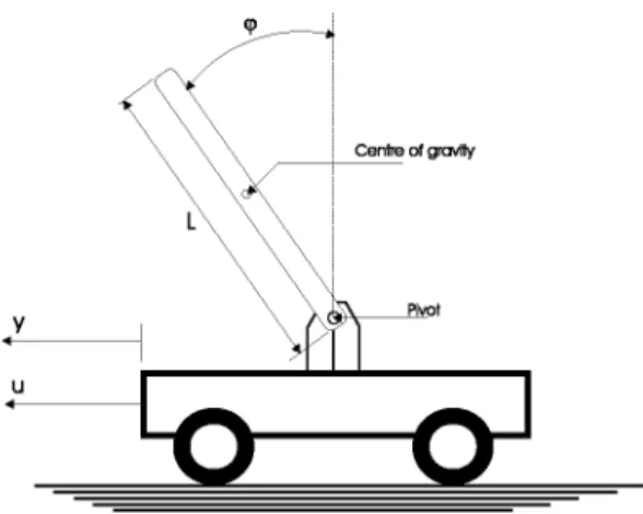
In this section, the proposed estimation method and its application to the control design of the FC-LQR is illustrated by an example of an inverted pendulum.

Consider the problem of stabilizing and balancing of swing up of an inverted pendulum (see Figure 2). The control of this system is a widely used performance measure of a controller, because this system is unstable and highly nonlinear. The objective is to maintain the inverted pendulum upright with 9 despite small disturbances because of wind or system noises.

The inverted pendulum can be represented as follows:

gsen9 — cos9( u+ml82sen8 \ M+m '

m

where 9 denotes the angular position (in radians) deviated from the equilibrium position (vertical axis) of the pendulum and 9 is the angular velocity, g(gravity acceleration) = 9 . 8 - ^ , M(mass) of the cart = 1 kg, m(mass) of the pole = 0.1 kg, 1 is the distance from the center of the mass (m) of the pole to the cart = 0.5 m.

Centre of grovtty

Assuming that xi 9 and x2 = 9, then (65) can be rewritten in state space form as follows:

xx =9

x{= x2

x2 = 9

x2

gsen(xx) - cos(x{)( T T2^ )

T / 4 mcos2(x\)\ " 3 M+m >

(66)

The aim is to move the pendulum to its unstable equilibrium position, that is, x\ = x2 = u = 0

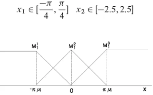
Firstly, the model of the inverted pendulum is estimated in three operation points for both the angle and its derivative. The universe of discourse of the angle is [-^, f ] rad, and one of the angu-lar velocity is [—5,5] r-f^. Both membership functions for the angle x and its derivative x are shown

seg

in Figures 3-4, respectively.

If we apply the T-S method directly to this example, then the condition number of the matrix X is 3.4148e + 015, which shows clearly a nonreliable result. Using the parameters' weighting method with weighting factor y = 0.01, the inverted pendulum fuzzy model can be represented as follows:

S12

s

s

s

s

s

s

s

If (xi is M / ) and If (xi is M / ) and If (xi is Mi) and If (xi is Mi) and If (xi is Mi) and If (xi is Mi) and If (xi is Mi) and If (xi is Mi) and If (xi is Mi) and

x2 is Mi)

x2 is M\)

x2 is M\)

x2 is M\)

then x2 = then x2 = then x2 = then x2 =

-8.1994 + 3.4151*1 - 0.2006x2

--8.3766 + 3.0426xi + 0.0000x2

--8.1994 + 3.4151xi + 0.2006x2

--0.0251 + 5.5416xi - 0.0085x2

-- 1.0443M

-1.0443M

-1.0443M

- 1.5332M

x2 is M2), then x2 = 0.0225 + 6.1796xi - 0.0000x2 - 1.5332w

x2 is Mi), then x2 = -0.0251 + 5.5416xi + 0.0085x2 - 1.5332w

x2 is Mi), then x2 = 8.1236 + 3.8634xi + 0.2363x2 - 1.0903w

x2 is Mi), then x2 = 8.0313 + 3.6645xi - 0.0000x2 - 1.0903w

x2 is Mi), then x2 = 8.1236 + 3.8634xi - 0.2363x2 - 1.0903

The resultant mean square error from this approximation is 0.0013. In this case, the condition number of the extended matrix Xa becomes 1.4569e +004, thus improving the reliability of results.

By using the identification with the classical minimum square method in an interval cióse to the equilibrium point,

Í I E [ J , ^ ] x2e [-2.5,2.5]

•Jl/4 0 » / 4 X

Figure 3. Membership functions for the angle x of the inverted pendulum.

The resultant linear model of the system in this interval is:

x2' = 0.0092 + 15.2665X! - 0.0000x2 - 1.4187w

This approximation gives us an idea of the quantitative relation among various variables. Compar-ing these parameters with those obtained in the previous fuzzy model, it is evident that its valúes are, in general, far enough from its physical ones. Moreover, if we compare the parameters of various adjacent subsystems, it can clearly verify that they are quite different.

By applying the tuning of parameters method, taking as a reference, the parameters obtained through minimum square method with a weighting factor y = 0.001 * np, where np is the number of samples used in the identification, we obtain:

0.1642 + 15.0162*1 - 0.3272x2 - 1.2458w

0.4847 + 14.6365x1 + 0.0000x2 - 1.1546w

0.1642 + 15.0162xi + 0.3272x2 - 1.2458w

-0.0064+15.4291x1 + 0.0171x2 - 1.4291w

-0.0796+15.5791x1 - 0 . 0 0 0 0 x2 - 1.4536w

:-0.0064+15.4291*1-0.0171*2-1.4291M -0.0927 + 15.1524xi+0.2813x2 - 1.3232M -0.2593 + 14.9994x1 + 0.0000x2 - 1.2568w

-0.0927+15.1524x1-0.2813x2-1.3232w

which has a mean square error of 0.0332 greater than the previous one but with more physical rela-tionship between variables. Nevertheless, as it can be seen that in this model a2,2 = —0.0796, which

does not fulfil an important characteristic of the existence of an unstable equilibrium point which is also the objective of control Xi = x2 = u = 0. In order that this point becomes an equlibrium in the

fuzzy model, a2,2 should be zero.

To achieve this target, we can either fix the valué of this parameter or assign it a very large weight-ing factor as explained in Section (4.2). In this case, a weightweight-ing factor of lOOy has been assigned to this parameter and finally the fuzzy model becomes:

s

s

s

s

s

s

s

s

s

(xi is M / ) (XI is M / ) (XI is M / ) (XI is M2)

(xi is M2)

(xi is M2)

(xi is M3)

(xi is M3)

(xi is M3)

and and and and and and and and and

\x2 is Mi),

\x2 is A f | ) ,

\x2 is Mi),

\x2 is Mi),

\x2 is Mi),

\x2 is Mi),

\x2 is Mi),

\x2 is Mi),

\x2 is Mi),

then x2

then X2 then X2 then x2

then X2 then x2

then X2 then x2

then X2

s

s

s

s

s

s

s

s

s

If (xi is M / ) and If (xi is Mi) and If (xi is Mi) and If (xi is Mi) and If (xi is Mi) and If (xi is Mi) and If (xi is Mi) and If (xi is Mi) and If (xi is Mi) and

xzisM;,1), then x2 = 0.1642+ 15.0164xi - 0 . 3 2 7 1 x2 - 1.2458w

x2 is Mi), then x2 = 0.4848 + 14.6366xi + 0.0002x2 - 1.1546w

x2 is Mi), then x2 = 0.1642 + 15.0162xi + 0.3272x2 - 1.2458w

x2 is Mi), then x2 = -0.0073+ 15.4272xi + 0.0172x2 - 1.4291w

x2 is Mi), then x2 = 15.5778xi - 0.0003x2 - 1.4536w

x2 is Mi), then x2 = -0.0072+15.4287xi - 0.0170x2 - 1.4291w

x2 is Mi), then x2 = -0.0001 + 15.1478xi + 0.3000x2 - 1.3232w

x2 is Mi), then x2 = -0.2646+14.9965xi + 0.0080x2 - 1.2568w

x2 is Mi), then x2 = -0.0942+15.1516xi - 0 . 2 8 2 1 x2 - 1.3232w

The minimum square error is 0.0333 which is slightly greater than that of the previous case but it represents the equilibrium point of the physical system, that is, a2,2 = 0. It can be clearly noticed in

this model that the distance between adjacent subsystem is relatively small. For each subsystem defined in the previous rules,

A feedback state LQR controller has been designed with the affine term:

Ahh) , iMih).

u = k%U2J + ky¡ll2>xl + k^'Áhh). 2'x2 + b(i^u

Firstly, the affine term of the controller is used to elimínate the affine term of the system

-a (hh) o fl(*l<2) + b(hi2)k(hh) = 0 = > k(hi2) _

o o o b(ni2)

The other terms are calculated by the LQR minimizing the following performance index:

/•OO

/ = / (IOOJCJ* + lOxf + u2)dt

Jt0

Thus, the resultant fuzzy optimal LQR is:

11 12 13 21 22 23 31 32 33

If (xi i s M / ) If (*i i s M / ) If (xi i s M / ) If (xi is M?) If (XÍ is M¡) If (xi is Mi) If (XÍ is M3)

If (X! is M¡) If (X! is M¡)

and and and and and and and and and

[x2 is M\),

[x2 is M | ) ,

'x

is

Mi),

[x2 is Mj1),

[x2 is M | ) ,

[x2 is M | ) ,

'x2 is M\),

\x2 is M^),

\x2 is M | ) ,

then u then w then u then M then u then M then w then u then M

= 0.1318 + 27.714ÓX! + 7.1239x2

= 0.4199 + 28.8232X! + 7.6493x2

= 0.1318 + 27.7153X! + 7.6493x2

= -0.0051 + 25.5103X! + 6.7723x2

= 25.3745^! + 6.7019x2

= -0.0050 + 25.5120X! + 6.7486x2

= 0.0001 + 26.6491X! + 7.321 lx2

= -0.2105 + 27.5014X! + 7.3389x2

= -0.0712 + 26.6529X! + 6.8812x2

It can also be noticed that the distance between the parameters of various adjacent control rules is relatively small. This in turn, strengths the hypothesis of designing a local control algorithm for each subsystem.

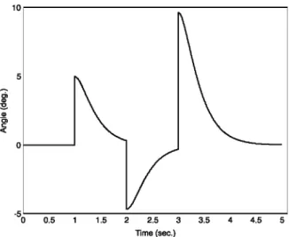
Figure 5 shows the controlled system behavior from an initial condition [j l]'. To examine the robustness of the proposed controller, it has been subjected to successive disturbance effects of 5o,

—5o, and 10° with respect to its equilibrium state as shown in Figure 6. It is clearly shown that

the inverted pendulum returns rapidly and smoothly to its equilibrium condition after applying each disturbance. Moreover, we have proven that the LQR is robust and invariant against measurement noise. If we suppose that the angle sensor introduces a noise of a = Io, it can be observed that the

output is only affected by a = 0.04° as shown in Figure 7. Figure 8 shows several trajectories in state space form of the system for several initial conditions.

1 1.5 2 Time (sec.)

Figure 6. Transient response of the inverted pendulum controUed by the fuzzy linear quadratic regulator subjected to successive disturbances.

Figure 7. Transient response of the inverted pendulum controUed by the fuzzy linear quadratic regulator subjected to measurement noise.

8. CONCLUSIONS

New efficient approaches have been presented to improve the local and global approximation of the T-S fuzzy model. The main problem of the T-S identification method is that it cannot be applied when the membership functions are overlapped by pairs. This restricts the use of the T-S method because this type of membership function has been widely used during the last 2 decades in the stability, controller design, and are popular in industrial control applications. The approaches devel-oped here can be considered as a generalized versión of the T-S method with optimized performance in approximating nonlinear functions. We propose a noniterative method through weighting of parameters approach and an iterative algorithm by applying the extended Kalman filter based on the same idea of parameters' weighting. We show that the Kalman filter is an effective tool in the identification of the T-S fuzzy model. An FC based LQR has been proposed in order to show the effectiveness of the estimation method developed here in control applications. An illustrative example of an inverted pendulum has been chosen to evalúate the robustness and remarkable per-formance of the proposed method and the high accuracy obtained in approximating nonlinear and unstable systems locally and globally in comparison with the original T-S model. Simulation results have shown the potential, simplicity, and generality of the algorithm.

REFERENCES

1. Takagi T, Sugeno M. Fuzzy identification of systems and its applications to modeling and control. IEEE Transactions

on Systems, Man, and Cybernetics 1985; 15(1): 116-132.

2. Gang F. A survey on analysis and design of model-based fuzzy control systems. IEEE Transactions on Fuzzy Systems 2006; 14(5):676-697.

3. Guerra TM, Vermeiren L. LMI-based relaxed nonquadratic stabilization conditions for nonlinear systems in the Takagi-Sugeno's form. Automática 2004; 40:823-829.

4. Lian K-Y, Su C-H, Huang C-S. Performance Enhancement for T-S Fuzzy Control Using Neural Networks. IEEE

Transactions on Fuzzy Systems 2006; 14(5):619-627.

5. Hseng T, Li S, Tsai S-H. Fuzzy bilinear model and fuzzy controller design for a class of nonlinear systems. IEEE

Transactions on Fuzzy Systems 2007; 15(3):494-506.

6. Chen B, Liu X, Tong S. Adaptive fuzzy output tracking control of MIMO nonlinear uncertain systems. IEEE

Transactions on Fuzzy Systems 2007; 15(2):287-300.

7. Jae-Hun K, Hyun C-H, Kim E, Park M. Adaptive synchronization of uncertain chaotic systems based on T-S fuzzy model. IEEE Transactions on Fuzzy Systems 2007; 15(3):359-369.

8. Zeng K, Zhang NY, Xu WL. A comparative study on sufficient conditions for Takagi-Sugeno fuzzy systems as universal approximators. IEEE Transactions Fuzzy Systems 2000; 8(6):773-780.

9. Johansen TA, Shorten R, Murray-Smith R. On the interpretation and identification of dynamic Takagi-Sugeno models. IEEE Transactions on Fuzzy Systems 2000; 8(3):297-313.

10. Tanaka K, Wang HO. Fuzzy Control Systems Design and Analysis: A Linear Matrix Inequality Approach. Wiley: New York, 2001.

11. Kóczy LT, Hirota K. Size reduction by interpolation in fuzzy rule bases. IEEE Transactions on Systems, Man, and

Cybernetics, Part B 1997; 27(1): 14-25.

12. Tikk D, Baranyi P, Patton RJ. Polytopic and TS models are nowhere dense in the approximation model space.

Proceedings of the International Conference on Systems, Man and Cybernetics (SMC'02), Hammamet, Tunisia,

2002.

13. Baranyi P, Korondi P, Hashimoto H. Global asymptotic stabilisation of the prototypical aeroelastic wing section via TP model transfromation. Asían Journal of Control 2005; 7(2):99—111.

14. Tikk D, Baranyi P, Patton RJ. Approximation properties of TP forms and its consequences to TPDC design framework. Asían Journal of Control 2007; 9(3):221-231.

15. Baranyi P, Szeidl L, Várlaki P, Yam Y. Definition of the HOSVD based canonical form of polytopic dynamic models. Proceedings of 3rd International Conference on Mechatronics (ICM 2006), Budapest, Hungary, 3-5 July 2006; 660-665.

16. Szeidl L, Várlaki P. HOSVD based canonical form for polytopic models of dynamic systems. Journal of Advanced

Computational Intelligence andIntelligent Informatics 2009; 13(l):52-60.

17. Baranyi P. SVD-based reduction to MISO TS models. IEEE Transactions on Industrial Electronics 2003; 51(l):232-242.

18. Matía F, Jiménez A, Al-Hadithi BM. An affine model with decoupled fuzzy dynamics, 22-27 June 2008; 713-720. 19. Cao SG, Rees NW, Feng G. Analysis and design for a class of complex control systems- Part I: fuzzy modeling and

20. Mollov S, Babuska R, Abonyi J, Verbruggen HB. Effective optimization for fuzzy model predictive control. IEEE

Transactions on Fuzzy Systems 2004; 12(5):661-675.

21. Skrjanc I, Blazic S, Agamennoni O. Interval fuzzy model identification using 1-Norm. IEEE Transactions on Fuzzy

Systems 2005; 13(5):561-568.

22. Klawonn F, Kruse R. Constructing a fuzzy controller from data. Fuzzy Sets and Systems 1997; 85(2): 177-193. 23. Hong TP, Lee CY. Induction of fuzzy rules and membership functions from training examples. Fuzzy Sets and

Systems 1996; 84(l):33-47.

24. Kim J, Suga Y, Won S. A new approach to fuzzy modeling of nonlinear dynamic systems with noise: relevance vector learning mechanism. IEEE Transactions on Fuzzy Systems 2006; 14(2):222-231.

25. Baranyi P, Korondi P, Patton RJ, Hashimoto H. Trade-off between approximation accuracy and complexity for T-S fuzzy models. Asían Journal of Control 2004; 6(l):21-33.

26. Tikk D, Baranyi P. Comprehensive analysis of a new fuzzy rule interpolation method. IEEE Transactions on Fuzzy

Systems 2000; 8(3):281-296.

27. Baranyi P, Kóczy LT, Gedeon TD. A generalized concept for fuzzy rule interpolation. IEEE Transactions on Fuzzy

Systems 2004; 12(6):820-837.

28. Yam Y, Wong ML, Baranyi P. Interpolation with function space representation of membership functions. IEEE

Transactions on Fuzzy Systems 2006; 14(3):398-411.

29. Yam Y, Kóczy LT. Representing membership functions as points in high dimensional spaces for fuzzy interpolation and extrapolation. IEEE Transactions on Fuzzy Systems 2000; 8(6):761Ü-772.

30. Kumar M, Stoll R, Stoll N. A min-max approach to fuzzy clustering, estimation, and identification. IEEE

Transactions on Fuzzy Systems 2006; 14(2):248-262.

31. Tao C, Taur J. Design of fuzzy controUers with adaptive rule insertion. IEEE Transactions on Systems, Man, and

Cybernetics-Part B: Cybernetics 1999; 29:389-397.

32. Simón D. Design and rule base reduction of a fuzzy filter for the estimation of motor currents. International Journal

ofApproximate Reasoning 2000; 25:145-167.

33. Wang L, Mendel J. Back-propagation of fuzzy systems as nonlinear dynamic system identiers. IEEE International

Conference on Fuzzy Systems, San Diego, California, 1992; 1409-1418.

34. Simón D. Training fuzzy systems with the extended Kalman filter. Fuzzy Sets and Systems 2002; 132:189-199. 35. Simón D. Sum normal optimization of fuzzy membership functions. International Journal of Uncertainty, Fuzziness

and Knowledge-Based Systems 2002; 10(4):363-384.

36. Wang L, Yen J. Extracting fuzzy rules for system modelling using a hybrid of genetic algorithms and Kalman filter.

Fuzzy Sets and Systems 1998; 101:353-362.

37. Hsiao C. Modified gain fuzzy Kalman filtering algorithm. JSME International Journal. Series C 1999; 42:363-368. 38. Kobayashi K, Cheok K, Watanabe K. Estimation of the absolute vehicle speed using fuzzy logic rule-based Kalman

filter. Proceedings of the American Control Conference, Seattle, WA, 21-23 Jun 1995; 3086-3090.

39. Jiménez A, Al-Hadithi BM, Matía F. An optimal T-S Model for the estimation and identification of nonlinear functions. WSEAS Transactions on Systems and Control 2008; 3(10): 897-906.

40. Kalman RE. A new approach to linear filtering and prediction problems. Transactions of the ASME. Series D, Journal

of Basic Engineering 1960; 82:35-45.

41. Gelb A. Applied Optimal Estimation. MIT Press: Cambridge, MA, 1974.

42. Lee TC, Yang DR, Lee KS, Yoon TW. Indirect adaptive backstepping control of a pH neutralization process based on recursive prediction error method for combined state and parameter estimation. Industrial and Engineering

Chemistry Research 2001; 40:4102-4110.

43. Puskorius G, Feldkamp L. Neurocontrol of nonlinear dynamical systems with Kalman filter trained recurrent networks. IEEE Transactions Neural Networks 1994; 5:279-297.

44. Jiang T, Li Y. Generalized defuzzification strategies and their parameter learning procedures. IEEE Transactions on