Design of a cylindrical near field system for radar antennas

DESIGN OF A CYLINDRICAL NEAR FIELD SYSTEM FOR RADAR ANTENNAS

Fernando Martín Jiménez, Sara Burgos Martínez, Manuel Sierra Castañer,

José Luis Besada Sanmartín

Grupo de Radiación. Dpto. SSR. Universidad Politécnica de Madrid ETSI Telecomunicación. Ciudad Universitaria. 28040 Madrid Spain

e-mail: [email protected]

Tel: +34913367360 Fax: +34915432002 Contact person: Fernando Martín Jiménez

ABSTRACT

A cylindrical near field measurement system for huge L-band RADAR antennas has been designed, and it is under construction. The cylindrical near field system consists of a 17 meters tower (15.5 meters linear scanning), placed at a distance between 4 and 7 meters from the centre of the RADAR antenna. The RADAR antenna is placed on its azimuth positioner, and the system must allow the measurement of the antenna without stopping the rotation movement, measuring two linear polarizations (horizontal and vertical). The system can work in both transmission and reception. The system must work in an open and windy area. To assure the rectitude of the z-axis, a servo controlled by an optical detector has been implemented.

This paper presents the main specifications of the measurement system (mechanical and electrical) and its design process. The paper will explain the acquisition routines (optimised for reducing measurement time without stopping the rotational movement of the RADAR), the control of the motors and RF equipment, the near field to far field transformation software, the algorithms used to compensate some errors (as temperature variations) and, finally, the user friendly environment.

1. INTRODUCCION

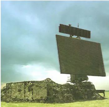
Huge antennas can not be measured in the standard near field or far field antenna measurement facilities. In this case, it is necessary to build an ad-hoc antenna measurement system to characterize L-band RADAR antennas. The RADAR antenna consists of linear dipole arrays up to 11 m, forming a plane structure close to 11x10 m similar to the one shown in Fig. 1. The system is complementary to the explained in [1], which is now working for testing each row of the array.

With this starting point, it has been designed an outdoor cylindrical measuring system. The system is based on a linear slide moving on a tower over 15m

height. The RADAR movement is used to perform the rotational movement.

Figure 1. Example of RADAR to measure.

The platform of the probe is exposed to the wind due to the height of the tower, and it produces measuring errors which are more important in phase. To reduce that error, it is required to assure the verticality of the probe movement, which means that the line described by the probe and the rotation axis of the RADAR are parallel. This requirement has been accomplished using a feedback loop based on a laser and an optical plummet.

In the following points these topics are described in detail together with the mean specifications (mechanical and electrical) of the system, the optimized movement cycles, the equipment employed and its control, the algorithm used to transform near to far field, and finally, the user friendly environment.

_____________________________________________________

Proc. ‘EuCAP 2006’, Nice, France

2. SYSTEM DESCRIPCION General specifications

The main specifications for the measuring system are: - Azimuthal angle range: 0º≤φ≤360º

- Elevation angle range: depends on the antenna geometry, the tower height and the distance between them.

- Gain maximum error: ±0.5 dB - Maximum error at -30 dB: ±2 dB - Maximum error at -40 dB: ±2 dB - Frequency range: 1000 to 1400 MHz

The geometric features of the measurement system: - Maximum utile shift for the probe along the tower:

15.5 m

- Distance probe-AUT (two positions): Maximum: 7 m Minimum: 4 m

Mechanical system

The mechanical system is based on a 17 m high tower. The probe platform moves along linear guides using rollers which assure a smooth movement with a position precision of +0.5mm and great repeatability. Moreover, the platform has a XY-table built by ourselves. This table has two motors that move the probe over rails for assuring the alignment of the system.

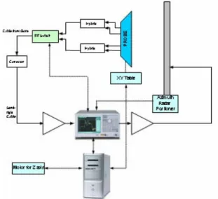
Radiofrequency system

The radiofrequency system is composed by:

- An Agilent network analyzer ENA E5070B, whose frequency range is: 300 KHz to 3 GHz.

- An electro-mechanical microwave switch from NARDA, controlled from the PC.

- Double polarized probe.

- RF Amplifiers for transmission and reception operation from MITEQ.

- Flexible RF cables from GORE optimized in length to maximize the system dynamic range.

Besides, the system must be able to work with the RADAR transmitting (Fig. 2) or receiving (Fig. 3).

3. POSITIONING SYSTEM

The system specifications listed before make necessary to develop an accurate positioning system. This problem has two aspects:

Positioning in Z axis (along the tower)

The probe in the Z axis is moved using a motor controlled by a PLC. The absolute z-position of the probe is controlled with a magnetic tape which is read by a magnetic lector.

Positioning in XY Plane (normal to the tower)

The positioning in this plane is the key point of the system. A study developed in [2] showed that the most important effect in the final results of a measurement of these kinds of RADAR is due to misalignments in x axis (from probe to AUT).

Figure 2. System operating with RADAR transmitting.

Figure 3. System operating with RADAR receiving.

This strategy is based on a laser beam that impinges on a circular quadrant detector. The signal returned by the detector is proportional to the deviation of the beam to the centre of the device. In fact, it returns one signal for x shift and another one for y shift, so it is possible to correct positioning errors in both axes.

These signals are sent to two PLCs that control a xy

motorized table. These devices make motors move trying to correct the beam deviation obtained from the detector output signals. When the beam impinges at the centre of the detector, the output signals are zero and the motors stop. Of course, the errors can be solved only while the beam is inside the range of the quadrant detector. Studies have shown that in normal operation (30 km/h wind) the deviations are lower than ±7 mm, and slow enough to be corrected by the laser loop.

So, if we have a stable laser beam perpendicular to the xy axes it is possible to ensure that the system is able to correct the errors by itself. These stability and perpendicularity are accomplished using an optical plummet.

4. ACQUISITION PROCESS

The acquisition process has several fixed parameters: RADAR rotation velocity, minimum number of sampling points to satisfy the sampling criterion, frequency of the measurement and angular range of validity. Due to these considerations, the measurement time will be really high.

The adopted strategy for data acquisition was to divide it into cycles of complete RADAR revolutions. The software routines were split into the PC and embedded macros in the ENA analyzer, which are much more time efficient.

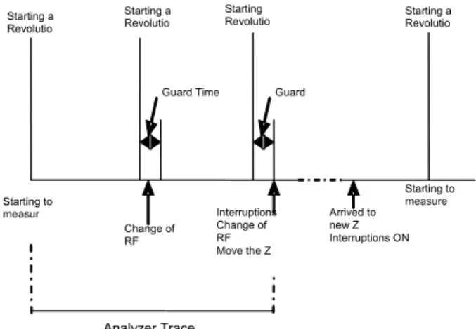
The RADAR azimuth positioner sends two signals: the most (starting of a RADAR revolution) and least significant bit of its angular resolution. The first signal determines the cycles explained before, according to Fig. 4. It arrives to the PC using the serial port as an interrupting signal. When one cycle starts, this interruption launches the measurement routine embedded in the Analyzer, which has been previously programmed at the beginning of the complete acquisition. The next interruption, observing a guard time, changes the RF switch controlled by the PC using the parallel port. Finally, the third interruption of the cycle, and again after a guard time, the interruptions are disabled, the probe is send to its new position in Z and the RF switch is changed to its first state. When the probe arrives to the aim position the interruptions are enabled again and the cycle restarts. Normally the probe movement can be completed in one RADAR

revolution, so the cycle is composed by three RADAR rotations.

Starting to measur

Starting a Revolutio

Starting a Revolutio

Change of RF

Guard Time Starting Revolutio

Guard

Interruptions Change of RF Move the Z

Arrived to new Z Interruptions ON

Starting a Revolutio

Starting to measure

Analyzer Trace

Figure 4. Time distribution for the measurement cycles

The analyzer embedded macro, once launched, take data at each sampling angle, using for triggering the less significant bit returned by the RADAR positioner. Like the angular resolution of the RADAR positioner is much more accurate than required, it is necessary to use a programmable frequency divisor (controlled by the PC in order to allow different number of sampling angles) before sending it to the Analyzer.

With the intention of adjusting as much as possible the time, the analyzer measures both polarizations in one trace. In this way, this trace will be composed by as many points as twice the angular sampling points plus the guard times. Thus, a post-process to obtain the definitive trace is compulsory. When a Z position has been finished, the data are saved to a file in the analyzer. Finally, when all the acquisition process is ended, this file is retrieved to the PC for its treatment.

5. TRANSFORMATION SOFTWARE

The method employed to establish the antenna far field pattern using probe near field measurement over the surface of a cylinder enclosing the antenna is based on

the scattering matrix formulation − see [3] and [4] −,

where different types of scattering matrices can be exploited to determine the coupling equation. The matrices are used to relate the amplitudes of waveguide modes to expansion coefficients by linear matrix transformations.

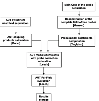
The near to far field conversion algorithm could be represented in the following diagram − see [4], [5], [6], [7] and [8]−:

AUT coupling products calculation

[Bucci] AUT cylindrical near field acquisition

AUT modal coefficients with probe correction

estimation [Leach]

Reconstruction of the complete field of two probes

[Hansen]

Probe modal coefficients computation

[Yaghjian] Main Cuts of the probe

acquisition

AUT Far Field evaluation [Leach] Results storage AUT coupling products calculation [Bucci] AUT cylindrical near field acquisition

AUT modal coefficients with probe correction

estimation [Leach]

Reconstruction of the complete field of two probes

[Hansen]

Probe modal coefficients computation

[Yaghjian] Main Cuts of the probe

acquisition

AUT Far Field evaluation

[Leach]

Results storage

Figure 5. Near to far field transformation algorithm.

So, to obtain the far field from the cylindrical near field measured, the following calculations are completed:

1. First, the AUT cylindrical near field is acquired and sampled.

2. Then, the AUT coupling products are calculated: T(n,h), where “n” is the number of modes and “h” is equal to k·cos θ (k = 2·π/λ).

3. After that, the reconstruction of the complete field of two probes, using the main cuts of the probe, is completed.

4. The next thing to do is the computation of the probe modal coefficients: c1(n,h), c2(n,h), d1(n,h), d2(n,h).

5. Afterwards, with the AUT coupling products and the probe correction coefficients, the AUT modal coefficients with probe correction can be determined: a(n,h), b(n,h).

6. Finally, the far-field of the AUT is established, normalized and stored: Eθ(r, φ, θ), Eφ(r, φ, θ):

∑

Eφ φ θ θ φ (1)

∑

( n 1

n n jn n jkr e k n b j r e k z r

Eθ φ θ θ φ(2)

7. Once the AUT far-field is known, the parameters of the AUT (radiated power, directivity…) can be deduced.

6. SOFTWARE INTERFACE

All the routines previously described are so complex that must be encapsulated in the most flexible and easiest way to be accomplished by any system operator. With this purpose, it has been implemented an user-friendly software environment that helps the system operation. This software, depicted at Fig. 6, allows the measurement and process definition, including: frequency or list of frequencies, polarization desired if it is only one required, type of RADAR, power to transmit, RADAR mode of operation (transmitting or receiving), acquisition points as well in azimuth as in Z axis, and RADAR rpm. Besides, it allows to acquire only at a concrete Z position or moving the probe without measuring.

Figure 6. Software interface main window.

7. CONCLUSIONS

A complete cylindrical antenna measurement system for huge RADAR antennas has been designed and now is under construction. All the system has been designed by a research group, with capabilities in antenna measurement: including radio frequency, mechanical components and software development. It is a really huge effort because of the enormous dimensions of the system to develop.

The effect of the alignment errors was simulated and then an automatic corrector system was implemented using a laser feedback loop that operates a

xy-table. The table reduces the error by means of a perpendicular laser plummet.

divided into the control PC and embedded macros in the analyzer in order to work in real time.

The software transformation from near cylindrical field to far field has been implemented by our research group, together with the measurement representation and data extraction routines. Finally, an user-friendly software environment has been performed to integrate all the routines involved in the measurement process, forming a complete and ease tool to control all the system.

8. REFERENCES

[1]. J. L. Besada, Fernando Martín, C. Martínez-Portas, M. Sierra-Castañer, M. Calvo Ramón, “A Linear Measurement System For Large Array Antennas”, AMTA symposium proceedings. Rodhe Island, USA. November 2005.

[2]. Sara Burgos, Fernando Martín, M. Sierra-Castañer, J. L. Besada, “Design and evaluation of a cylindrical near field system for RADAR antennas”, AMTA Europe symposium proceedings, Munich, Germany, May 2006.

[3]. Jorgen Appel Hansen, “On cylindrical near field scanning techinques”, IEEE transactions on antennas and propagation, vol. ap-28, no. 2, pp. 231-234, March 1980.

[4]. Arthur D. Yaghjian, “An overview of near field antenna measurements”, IEEE transactions on antennas and propagation, vol. ap-34, no.1, pp. 30-45, January 1986.

[5]. W. Marshall Leach, Jr. and Demetrius T. Paris, “Probe Compensated Near Field Measurements on a Cylinder”, IEEE Transactions on Antennas and Propagation, Vol. AP-21, No. 4, pp. 435-445, July 1973.

[6]. Z. A. Hussein, Y. Rahmat-Samii, “Probe Compensation Characterization in Cylindrical

Near-Field Scanning”, IEEE, pp. 1808-1811, 1993. [7]. O. M. Bucci, “Use of Sampling Expansions in

Near-Field-Far-Field Transformations: The Cylindrical Case”, IEEE Transactions on Antennas and Propagation, Vol. 36, No. 6, pp. 830-835, June 1988.