Error estimations in cylindrical near field system for large radar antennas

ERROR ESTIMATIONS IN CYLINDRICAL NEAR FIELD SYSTEM FOR LARGE

RADAR ANTENNAS

S. Burgos (1)_{, F. Martín} (1)_{, M. Sierra-Castañer} (1) _{and J.L.Besada} (1)

(1)_{Grupo de Radiación. Dpto. de Señales, Sistemas y Radiocomunicaciones.}

Univ. Politécnica de Madrid. E.T.S.I. de Telecomunicación. Ciudad Universitaria. 28040 Madrid. Spain Tel.. +34913367366 ext. 4053 Fax.. +34915432002

Email:[email protected], [email protected], [email protected], [email protected]

ABSTRACT

Cylindrical near field systems are appropriate measurement systems for huge L-band RADAR antennas, because the antenna can be measured on its azimuthal positioner and the probe can be easily translated through a vertical linear slide. So for large antennas the mechanical aspects of the antenna measurement systems are important and the errors in this mechanical part can affect to the far field radiation pattern.

This paper presents an error estimation tool to analyze the most important errors in one cylindrical acquisition system and the effect of these errors in the calculation of the far field radiation pattern. This study has been performed to improve the cylindrical system and to evaluate the error budget of the Antenna Under Test (AUT). The simulator calculates the far field from an array of dipoles over a ground plane (Antenna Under Test model) and compares the ideal result with the electric field obtained using the cylindrical near to far field transformation algorithms.

The results achieved are the variation in the principal patterns of the far field, RMS errors in side lobes and maximum errors in side lobes. Random and deterministic source of errors have been considered. 1. INTRODUCTION

Large antennas need special measurement system. This paper presents a measurement system for large L-band RADAR antennas. These antennas have the possibility of operating with a sum or a difference pattern. The maximum length of the array antennas (up to 12 meters) requires an especially long antenna measurement system. The designed system is a cylindrical near field range, where the RADAR antennas rotates on its own positioner, and the probe (double-polarized probe) moves along a 15.5 meters linear slide, stopping in each of the defined position to acquire the near field. Besides, the antenna can work in reception and transmission.

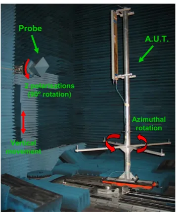
To realize how big the measurement system has to be, the following picture (Fig.1) represents one possible Antenna Under Test to evaluate.

The acquired field is then processed, employing cylindrical near to far field transformation techniques, to obtain the far field radiation pattern and the gain. Afterwards a post processing is performed to recover the radiation pattern main parameters. This paper is focused on the evaluation of the main errors that affect the radiation pattern. The errors are due to mechanical misalignment of the system, to phase errors caused by temperature variations and errors due to the S/N in the receiver.

Figure 1. Example of an Antenna Under Test

This paper is divided in following parts. First, section 2 describes the main characteristics and specifications of the measurement system. After that, section 3 explains the cylindrical near to far field transformation software. Next, section 4 validates the method applied. Afterward, section 5 exposes the main source of errors to analyze and the solutions implemented to reduce them. Then, section 6 comments the error simulator designed and the results. And finally, section 7 mentions the conclusions.

_____________________________________________________ Proc. ‘EuCAP 2006’, Nice, France

2. MAIN SPECIFICATIONS OF THE MEASUREMENT SYSTEM

The main specifications of the measurement system evaluated are:

− Maximum size of the Antenna under Test (AUT): length = 12 meters and height = 7.5 meters. − Frequency range: L band, 1215 – 1400 MHz. − Maximum length of the linear slide: 15.5 meters. − Distance from AUT to Probe: between 4 and 7

meters.

− Azimuth angular range: 0º ≤φ≤ 360º.

− Elevation angular range: depends on geometry of the system and antenna.

− Antenna under Test: arrays of dipoles with uniform, Taylor or Bailyss amplitude distribution in both vertical and horizontal planes, and different in reception or transmission performance. − Minimum Rotation velocity of the AUT (velocity

for measurement process): 5 – 7.5 rpm. − Measurement errors:

o Maximum error in gain: ± 0.5 dB.

o Error at – 30 dB SLL: ± 2 dB.

o Error at – 40 dB SLL: ± 3 dB.

o Pointing error: ± 0.05º in both azimuth and elevation planes.

The system has been designed to assure the previous errors in the frequency band, and this study analyses the effect of the previous errors in final results of the radiation pattern.

This first analysis has been performed considering a theoretical antenna (Antenna Under Test and probe), whose main characteristics are:

- Length: 2.52 meters (14 columns). - Height: 2.08 meters (16 rows).

- Radiating element: vertical λ/2 dipole over a ground plane.

- Columns excitation: uniform in amplitude and phase.

- Rows excitation: tapered in amplitude and uniform in phase.

- Distance from antenna to probe: 4 meters. - Probe: ideal horn cos3_{θ, which can perform a}

polarization rotation on its positioner. - Length of the vertical slide: 15.5 meters. - Frequency: 1215 MHz.

- Cylindrical Near field acquisition: 128 angular positions and 125 vertical positions (samples separated 12.5 cm (≈λ/2).

In the following figures, a practical (Fig.2) illustration of the studied system is represented:

Probe

A.U.T.

Azimuthal rotation

Vertical movement

2 polarisations (90º rotation)

Probe

A.U.T.

Azimuthal rotation

Vertical movement

2 polarisations (90º rotation)

Figure 2.Practical illustration of the system

3. CYLINDRICAL NEAR FIELD TO FAR FIELD TRANSFORMATION

The method employed to determine the antenna far field pattern from probe compensated near field data measured over the surface of a cylinder enclosing the antenna is based on the scattering matrix formulation

− [1], [3] −, where different types of scattering matrices can be used to derive the coupling equation. The matrices are used to relate the amplitudes of waveguide modes to expansion coefficients by linear matrix transformations. These matrices can be taken as definitions or derived from Maxwell’s equations.

In order to perform a precise measurement, it has to be considered that the probe employed to measure has an impact on the samples retrieved. Therefore, a probe correction has to be carried out, so as to compensate this undesired side-effect.

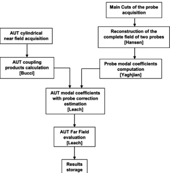
The near to far field conversion algorithm is represented in the following diagram (Fig.3) − [2], [3], [4], [5], [6], [7], [8], [10] −:

AUT coupling products calculation

[Bucci] AUT cylindrical near field acquisition

AUT modal coefficients with probe correction

estimation [Leach]

Reconstruction of the complete field of two probes

[Hansen]

Probe modal coefficients computation

[Yaghjian] Main Cuts of the probe

acquisition

AUT Far Field evaluation [Leach] Results storage AUT coupling products calculation [Bucci] AUT cylindrical near field acquisition

AUT modal coefficients with probe correction

estimation [Leach]

Reconstruction of the complete field of two probes

[Hansen]

Probe modal coefficients computation

[Yaghjian] Main Cuts of the probe

acquisition

AUT Far Field evaluation

[Leach]

Results storage

Figure 3. Near to far field transformation algorithm

So, the transformation process is divided in the following steps:

1. First, the AUT cylindrical near field is acquired and sampled.

2. Then, the AUT coupling products are calculated: T(n,h), where “n” is the number of modes and “h” is equal to k·cos θ (k = 2·π/λ). They are calculated through a FFT in azimuthal dimension and a DFT in vertical range (values for a regular grid in θ

angles are obtained in the valid angular range). 3. After that, the reconstruction of the complete

field of two orthogonal linear polarized probes, using the main cuts of the probe, is completed. The probes satisfy µ=±1.

4. The next thing to do is the computation of the probe modal coefficients: c1(n,h), c2(n,h), d1(n,h),

d2(n,h) through an inverse FFT.

5. Afterwards, with the AUT coupling products and the probe correction coefficients, the AUT modal coefficients with probe correction can be determined: a(n,h), b(n,h).

6. Finally, the far-field of the AUT is established, normalized and stored: Eθ(r, φ, θ), Eφ(r, φ, θ):

∑

E_φ φ θ θ φ (1)

∑

Eθ φ θ θ φ (2)

7. Once the AUT far-field is known, the parameters of the AUT (radiated power, directivity, beamwidth…) can be deduced.

4. METHOD VALIDATION

In order to validate this formulation, a comparison between the theoretical far field and the far field obtained after processing an ideal cylindrical acquisition has been performed, as it is illustrated in the next graph (Fig.4):

Near To Far Field

Near To Far Field

TRANSFORMATION

TRANSFORMATION (with probe correction)

Far Field Radiation Pattern COMPARISON IDEAL Acquisition THEORETICAL FIELD

THEORETICAL FIELD: •Array Factor

•Dipole radiation pattern in the main planes

Far Field Radiation Pattern

Near To Far Field

Near To Far Field

TRANSFORMATION

TRANSFORMATION (with probe correction)

Far Field Radiation Pattern Far Field Radiation Pattern COMPARISON IDEAL Acquisition THEORETICAL FIELD

THEORETICAL FIELD: •Array Factor

•Dipole radiation pattern in the main planes

Far Field Radiation Pattern

Far Field Radiation Pattern

Figure 4. Validation Diagram

The theoretical far field has been calculated multiplying the array factor by the λ/2 dipole radiation pattern. On the other hand, the ideal acquisition has been performed on a cylinder whose radius is 4 meters and whose generatrix is 15.5 meters.

Besides, the received field in each point of the grid has been calculated, considering the field radiated by all the dipoles modified by the probe pattern.

The field from each dipole in a point of the grid is given by the sum of 3 plane waves modified by the probe radiation pattern in the appropriate direction [9]:

( ) ( ) ( )_⎟⎟ ⎠ ⎞ ⎜⎜ ⎝ ⎛ θ − θ + θ

= − − − s

jkr 1 2 x 2 jkR 1 s 1 jkR mn z f r e ) kL cos( 2 f R e f R e I

E 1 2 (3)

where the angles and distances are shown in Fig.5, and fs is the radiation pattern of the probe:

I(z )

zd 2= -L1

zd 1= L1

z

P R O B E : P (x , y , z )

x r R2 R 1 θ2 θ1 θ

D IP O L E I(z )

zd 2= -L1

zd 1= L1

zz

P R O B E : P (x , y , z )

x r R2 R 1 θ2 θ1 θ

D IP O L E

Besides, as the parameter “L1” is equal to λ/4 (half

wavelength dipole), therefore the expression of the radiated field is simplified (4), and the probe radiation pattern is cos3_θ:

_⎟⎟

⎠ ⎞ ⎜⎜

⎝ ⎛

θ +

θ

= − − 2

3

2 jkR

1 3

1 jkR

mn

z _R cos

e cos R e I

E 1 2 (4)

Furthermore, in order to make the calculation of the field easier, the “Image Theory” is applied to the parallel dipoles array of the AUT.

Fig. 6 and Fig. 7 represent the comparison in the main planes between the theoretical far field and the far field obtained in two steps: first after an ideal acquisition and then a cylindrical near to far field transformation.

Figure 6.Comparison of theoretical far field and ideal transformed far field. Horizontal plane

Figure 7. Comparison of theoretical far field and ideal transformed far field. Vertical plane

The slight error observed in the vertical plane is due to the fact that the number of samples evaluated in the vertical axis, “z-axis” of the probe, is finite.

5. SOURCES OF ERRORS ANALYSIS

The main errors that affect to a near field measurement range are summarized in [10] ,[11] , [12].

The most important error sources for our case of study (outdoor facility) are:

- RF Measurement system: Dynamic range and random amplitude and phase.

- Positioning system: mechanical positioning and probe orientation/rotation.

- Near field probe: mechanical alignment and scattering cross section.

- Environmental: Temperature, temperature spatial gradient, electromagnetic interference and reflections.

- Measurement procedure: limited measurement area, sample point spacing, sampling time rate and Probe/AUT separation (multiple reflections).

- Computational: algorithm approximations.

In section 4 the computational errors and the errors due to limited measurement area and sample point spacing are observed in the comparison between the theoretical far field and the ideal transformation from near to far field. These errors are negligible in the horizontal plane. However, in vertical plane some errors are observed in the extreme angles.

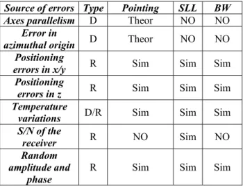
This paper analyses the errors in the beamwidth, directivity, SLL and pointing direction for the sources of errors shown in Tab. 1 (notice that there are some important errors as the reflections that are not analysed). The type of error is “R” (random) or “D” (deterministic). The 3 last columns show the methods employed to evaluate the errors: “NO” means that the error is not important, “Theor” indicates that the effect of the error can be estimated theoretically and “Sim” denotes the effect of the error is evaluated by simulation.

Source of errors Type Pointing SLL BW Axes parallelism D Theor NO NO

Error in

azimuthal origin D Theor NO NO Positioning

errors in x/y R Sim Sim Sim Positioning

errors in z R Sim Sim Sim Temperature

variations D/R Sim Sim Sim S/N of the

receiver R NO Sim NO

Random amplitude and

phase

R Sim Sim Sim

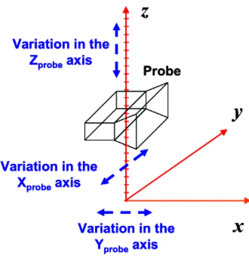
The positioning errors in x and y direction can be very important because of the windy outdoor conditions.

Therefore, an analog servo have been designed to reduce these errors. A laser impinges on a quadrant detector and two signals (one for each direction) are obtained. These two signals excite both PLC that control the x and y positions of the probe (installed over a xy double slide). The residual errors in these directions are estimated in ± 1 mm. The effect of these errors are evaluated through simulations.

The positioning errors in z direction are due to thermal expansions and positioning errors (encoder, PLC …). These errors are estimated in ± 0.5 mm.

y

z

x

Zprobeaxis

Variation in the Xprobeaxis

Variation in the Yprobeaxis

Probe

y

z

x

Zprobeaxis

Variation in the Xprobeaxis

Variation in the Yprobeaxis

Probe

Figure 8. Positioning errors studied

The temperature variations during a measurement (around 90 minutes) can be estimated in 10ºC. This shift can produce up to 8 degrees in the variation of the phase. The system cannot support this high deviation, so it must be rectified. The correction procedure consists in measuring several times the same position (central position) during the acquisition, obtain the variation (a complex factor) due to temperature changes in the 5 times, and interpolate this correction factor for all the times. Each acquired value is corrected with this term. With this correction the error is estimated in ± 1 deg.

The S/N in the receiver is evaluated for the effect on the lobe Side levels. The effect is accomplished adding a random noise to each value of the acquired field. For the estimations, a dynamic range in the maximum equal to 75 dB (theoretical value) is considered. This error cannot be corrected.

Other possible errors consist in including a random amplitude and phase in each point. A random value equal to ± 0.1 dB in amplitude and ± 3 degrees in phase is considered in the error calculations.

6. ERROR SIMULATOR

The simulation process performed can be represented in the following diagram (Fig.9):

CNIFT (Near-To-Far Field

Transformation)

Acquisition with ERRORS

Far field Radiation Pattern

COMPARISON IDEAL

Acquisition

CNIFT (Near-To-Far Field

Transformation)

Far field Radiation Pattern CNIFT

(Near-To-Far Field Transformation)

Acquisition with ERRORS

Far field Radiation Pattern Far field Radiation

Pattern

COMPARISON IDEAL

Acquisition

CNIFT (Near-To-Far Field

Transformation)

Far field Radiation Pattern Far field Radiation

Pattern

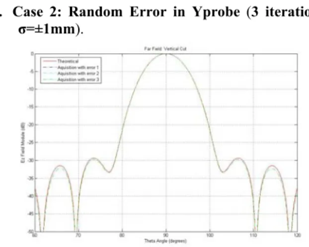
Figure 9. Diagram of the simulation process From all the scenarios studied we represent the most relevant ones. First, Fig. 10 and Fig. 11 shows the effect of a variation in x position of the probe in vertical and horizontal planes. Then, Fig. 12 represents the error in y position in the vertical plane and finally, Fig. 13 and Fig. 14 illustrate the error in amplitude and phase in the horizontal and vertical plane.

1. Case 1: Random Error in Xprobe (3 iterations,

σ=±1mm).

Figure 10. Random error in Xprobe, Horizontal plane.

2. Case 2: Random Error in Yprobe (3 iterations,

σ=±1mm).

Figure 12. Random error in Yprobe, Vertical plane.

3. Case 3: Random Error in Amplitude and Phase (3 iterations, σ=±0.1dB and σ=±3º).

Figure 13. Random error in Amplitude and Phase, Horizontal plane.

Figure 14 Random error in Amplitude and Phase, Vertical plane..

7. CONCLUSION

A cylindrical near to far field transformation software for a L-band RADAR antenna measurement system has been implemented and evaluated through simulations.

Furthermore, a detailed analysis of the main source of errors in this outdoor range has been performed, and some errors have been corrected using some algorithms or optical systems (based on a laser, a quadrant detector and an analogue servo).

For other sources of errors a Montecarlo simulator is prepared, and the first simulations are carried out. The primary analysis of the results show that the main sources of errors are due to x variation in the position of the probe (bigger effect than y or z variation) and the errors in amplitude and phase (random noise added to the signal).

This study is going to be completed with a large number of simulations, including the different errors, and the results will be presented in the symposium. These results will show a quantified error on different parameters: beamwidth, SLL, directivity and pointing direction.

ACKNOWLEDGEMENT

The authors want to acknowledge the support from INDRA Sistemas for the development of this work. REFERENCES

[1] Jørgen Appel Hansen, “On Cylindrical Near-Field Scanning Techniques”, IEEE Transactions on Antennas and Propagation, Vol. AP-28, No. 2, pp. 231-234, March 1980.

[2] W. Marshall Leach, Jr. and Demetrius T. Paris, “Probe Compensated Near Field Measurements on a Cylinder”, IEEE Transactions on Antennas and Propagation, Vol. AP-21, No. 4, pp. 435-445, July 1973.

[3] Arthur D. Yaghjian, “An Overview of Near-Field Antenna Measurements”, IEEE Transactions on Antennas and Propagation, Vol. AP-34, No. 1, pp. 30-45, January 1986. [4] J. J. Serrano Bermejo, “Software para la conversion de campo

próximo cilíndrico a campo lejano incluyendo corrección de sonda. Master Thesis. September 2003.

[5] W. Rudge, K. Milne, A.D. Olver and P. Knight, “The Handbook of Antenna Design”, Vol 1, 1982, pp. 609-614.

[6] Alan V. Oppenheim, Alan S. Willsky with Ian T. Young, “Signals and Systems”, Ed. Prentice-Hall International Editions. [7] O. M. Bucci, “Use of Sampling Expansions in Near-Field-Far-Field Transformations: The Cylindrical Case”, IEEE Transactions on Antennas and Propagation, Vol. 36, No. 6, pp. 830-835, June 1988.

[8] Z. A. Hussein, Y. Rahmat-Samii, “Probe Compensation Characterization in Cylindrical Near-Field Scanning”, IEEE, pp. 1808-1811, 1993.

[9] Robert S. Elliot, “Antenna Theory and Design”, Ed. Prentice-Hall, Inc., Englewood Cliffs, New Jersey.

[10] Jørgen Appel Hansen, “Spherical Near-Field Antenna Measurements”, Edited by J. E. Hansen and published by Peter Peregrinus Ltd., on behalf of IEE, London, United Kingdom, 1988.

[11] Edward B. Joy, “Near-Field Rang Qualification Methodology”, IEEE Transactions on Antennas and Propagation, Vol. 36, No. 6, pp. 836-844, June 1988.

[12] A.C. Newell, “Error Analysis Techniques for Planar Near Field

Measurements”, IEEE Transactions on Antennas and