Mathematical analysis of a model of
chemotaxis arising from morphogenesis
Christian Stinner, J. Ignacio Tello and Michael Winkler
Communicated by H.A. Levine
We consider non-negative solution couples (u, v) of
ut = uxx-x(^vx)x-Xu, vt = 1 — V + u,
with positive parameters / and X, where the spatial domain is the interval (0,1). This system appears as a limit case of a model for morphogenesis proposed by Bollenbach et al. (Phys. Rev. E. 75,2007). Under suitable boundary conditions, mod-eling the presence of a morphogen source atx = 0, we prove the existence of a global and bounded weak solution using an approximation by problems where diffusion is introduced in the ordinary differential equation. Moreover, we prove the convergence of the solution to the unique steady state provided that / is small and X is large enough.
Numerical simulations both illustrate these results and give rise to further conjectures on the solution behavior that go beyond the rigorously proved statements. Copyright © 2012 John Wiley & Sons, Ltd.
Introduction
Chemotaxis is a phenomenon present in many different biological processes where cells and other micro-organisms orient their move-ment by an external chemical signal, moving towards the direction of the gradient of the concentration of the chemical substance. Some of the biological processes involving chemotactic movement are, for instance, bacteria movement, immune response,
vascu-larization, one of the key processes in tumor growth, wound healing or Morphogenesis. The process of Morphogenesis (the creation,
"genesis" of shapes, "morphe") has been studied since the early 20th century. It occurs in the formation of the embryo and is responsible for the differentiation of the cells to create organs and their organization. During the process, the cell receives a chemical signal -the "morphogen"-which binds to -the receptors of -the cell situated on its surface. The cell monitors -the concentration of morphogens received and activates its differentiation. The morphogens are secreted at localized signaling sites, and how they are transported to the cells of the embryo is a controversially discussed question. Theoretical and experimental scientists have considered different possibil-ities: transport of morphogens by diffusion in the extracellular matrix of the embryo or transport by contact between cells. In the last decade, several authors have considered mathematical models of partial differential equations (see for instance [1 -9]) where diffusion is considered totally or partially responsible of the transport. Recently Bollenbach etal. [10] have introduced a mathematical model to describe the transport of morphogens in Epithelia. In [10], a system of PDEs is presented where the transport of morphogens is induced not only by diffusion, but also by the gradient of the concentration of receptors. Chemotactic terms in morphogen transport have been also considered in Merkin etal. [11],
The mathematical model proposed in [10] for the transport in large time scales consists of a system of two equations: A PDE of parabolic type models the time evolution of the total ligand density u, and an ODE describes the behavior of the free and bound receptor density v. A general form of the spatially one-dimensional version of this model reads
ut = (d] (u, v)ux - d2(u, v)vx)x - K-\ (u, v)u, x e (0,1), f > 0,
where di(u,v) is the diffusion coefficient, djiu,v) is the coefficient of morphogen transport induced by the gradient of the receptor concentration, K-\(U,V) and K2(u,v) are the degradation rates of the morphogen and receptor, respectively, and vsyn describes the receptor production at the surface of cells. In order to close the problem mathematically, we have to introduce appropriate boundary conditions and initial data. A t x = 0, the flux through the boundary is related to the production rate at the signaling site, that is,
du dv
di(u,v)- d2( u , v ) — = v a t x = 0, (2)
an an
where n is the outward unit normal. At x = 1, zero flux boundary conditions are imposed, that is,
I— -d2(u,v) — dn dn
d i ( u , v ) / - d2( u , v ) / = 0 a t x = 1 . (3)
Bounded non-negative initial data
u(x, 0) = u0 (x), v(x, 0) = v0 (x) (4)
are assumed to be known.
The coefficients considered in [10] are given by
A f ^ D l V A f ^ °2" , .^ K3V-K4U
di("'v) : = T. T^' d2(u,v) := — , K2(U,V) : = , (5)
b-\u + b2V b-\u + b2V v
and a constant degradation rate K-\ is assumed there. The receptor production term vsyn is proposed in [10] to be a linear function of the receptors and the blind receptors, that is, vsyn = OQ + a-\V + ajv, where v and v are the free and the blind receptor concentration. For further details in the modeling, we refer the reader to [10]. In this paper, we assume that
1. v and v depend linearly on uand v, that is, vsyn is given by vsyn = OQ + a-\V + aju with certain constants OQ, a-\, and aj. 2. In (1) and (5) we have b-\u « bj\i.
3. For the constants in (5) and 1, we have «i < K-$.
After re-normalizing the system and assuming , , Pl__ . = 1 and QQ = 1,(1)-(4) is simplified to
"r = uxx-x (-vx) - Au, x e (0,1), r > 0, vt = 1 - v + u, x e (0,1), r > 0,
u u (6) ux — x~vx = —v, x = 0, f > 0, ux — x~vx = 0, x = 1, f > 0,
u(x,0) = u0(x), V(X,0) = v0(x), x e (0,1), where A := K l- > 0, v > 0, and we assume y e (0,1).
In this paper we, consider the system (6) and study the well-posedness of the problem under mild assumptions on the initial data. The main results of the paper concern global existence and boundedness of weak solutions (see Lemma 2.6 and Lemma 2.7), as well as asymptotic stability of the unique steady state for a range of parameters (see Theorem 4.1). A regularization method is consid-ered to study the problem, where diffusion is introduced in the ODE. When the diffusion coefficient goes to zero the solutions of the approximating problem indeed approach a solution of (6).
Before going into details, let us establish some further connection to the existing literature. We first note that mathematical aspects of morphogenesis models have been considered by several authors. For instance, Merkin etal. [11] have introduced a chemosensitivity term in the model to describe morphogen concentration. They have presented results on the existence and uniqueness of classical and self-similar solutions to the corresponding system. Their numerical simulations have shown periodic pulse solutions. Mathematical analysis of models of morphogenesis has also been presented in Krzyzanowski etal. [4], where convergence of associated solutions to steady states is studied. Krzyzanowski etal. [5] also considered a mathematical model with nonlinear diffusion and without chemotac-tic term. The authors present their model and study the steady states, numerical simulations show the sensitivity of the solutions with respect to some parameters.
Next, viewing (6) from a mathematical point of view, one observes that as a consequence of the limit procedure included in our modeling, the "chemotactic sensitivity" / ( u , v), chosen as / ( u , v) := x • 7 in (6), becomes singular at zeros of v. Singular chemotactic sensitivity functions of this type have been considered in various models for chemotaxis processes other than morphogen transport (cf. [12,13] and the survey [14], for instance). These and related works seem to indicate that the analysis of chemotaxis models with such sensitivity functions is more delicate than in neighboring regular situations [14-17],
Throughout this paper, we define Q : = (0,1),assume A > Oand v > Oand require that the initial data satisfy
UQ,VQ eC^(Q), UQ>0, and VQ > 0 in Q. (7)
1. Preliminaries and approximation of solutions
In this section, we first introduce the definition of a global weak solution of (6). This weak solution will be obtained through approxi-mation by solutions of certain regularized problems. The existence of classical solutions to the approximate problems will also be part of this section.
Definition 1.1
let x > O.Then by a global weak solution of(6), we mean a couple (u,v) of functions
and
u € /.£(« x [o,oo)) n /^(p,oo); IV
1'
1(«))
v e L j £ ( S x p , oo)) n Lj£([0, oo); IV1-1 ( « ) ) ,
such that u > 0 and v > 0 a.e. i n f i x (0, oo), and such that the identities
- / m~ u0(x)<p(x,0)dx = - / ux(px + x / -vx(px
JO JQ JQ JO JQ JO JQ v
/•OO / > 0 0 /• +v / ^ ( o , r ) d r - A / I u<p
Jo Jo JQ
and
- / V(Pt~ v0(x)<p(x,0)dx = / I (\-v + u)<p Jo Jo. JQ JO JQ
hold for all cp e C°°(fi x [0, oo)).
In order to construct a weak solution of (6) in a convenient way, let us consider the parabolic-parabolic regularization of (6) given by
Uet = Usxx - X (vZvex) ~ Au«, X € ( 0 , 1 ) , f > 0, Vet = SVexx + 1 - Ve + Ue, X € ( 0 , 1 ) , f > 0,
Uex = — v, vex = 0, X = 0, f > 0, Uex = Vex = 0, X = 1, f > 0,
Us (x, 0) = U0 ( x ) , Vs (x, 0) = V0 ( x ) , X € ( 0 , 1 ) ,
(8)
for B€ (0,1).
Using arguments similar to those in [18] and [16], we now show the local existence and uniqueness of solutions to (8).
Lemma 1.2
L e t / > 0, e e (0,1), q > 1,u0 e C°(S2) and v0 e U A ^ f i ) such that (7) is fulfilled. Then there exists 7"g e (0,oo] and a pair (ue,ve) of functions
ug e C°([0,7g); C°(S)) n C2'1 (Q x (0,7",)),
/g e C°([0,7,); C°(£2)) n Z.j£([0,7i); I V1* ^ ) ) n C2'1 ( 6 x (0,7",)),
which solves (8) in the classical sense. If Te < oo then
l l " « ( 0 l k ~ ( Q ) + I I ^ ( O I I M / I . I ( Q ) ^ o o as t/Te. (9)
Moreover, (ue,ve) satisfies
us > 0 in £2 x[0,7g), (10)
yg > min <1,min vo(x)f =:co > 0 in fi x [0,7~g), ( X € Q
(11)
/ us(x, f ) d x < max < /
JQ [J& Q A I U0, - > = :'f1 f o r a" t G (°<7s)<
and
/ Vg(x, f ) d x < m a x ] / v0,1 + k-\ \ =:c-\ for all r e (0, Te). JQ UQ )
(13)
Proof
We fix B e (0,1). In order to cope with the boundary conditions and the singularity in the first equation of (8), we set (p(x) := -vx(l — x )2, x e £2, and choose a nondecreasing function p e C1 + a( R ) such that
P(s) s 4
f o r s > f , f o r s < ^ ,
where a is positive and Co is defined in (11). If (ue,Vg) is a solution of
Ugt = usxx - x (jtfyvex) ~ Xu?' x e (0,1), r > 0, Vgt = evexx + 1 - Vg + Ug, x e (0,1), r > 0,
uex = — v, vex = 0, x = 0, f > 0, uex = vex = 0, x = 1, f > 0, Ug (x, 0) = u0 (x), Vg (x, 0) = v0 (x), x e (0,1),
(14)
then (ue,Vg), where ue(x,t) := ue(x,t) — (p{x), is a solution of the problem
Ugt •• uexx - x (^jVex) - Mug + <p) + <pxx, x e (0,1), r > 0, eVgXX + 1 - Vg + Ug + (p, x € (0,1), r > 0,
Vgt
uex = vex = o,xe {0, l } , r > 0,
ug(x,0) = u0(x) - (p(x,0) =: u0(x), ve(x,0) = v0(x), x e (0,1).
(15)
To obtain a solution of the latter problem, we let B := {(us, vs) e X : X : = C°([0,T];C0(Q)) x L°°([0,T]; W^(Si)) equipped with the norm \\(ue,ve and R are positive constants. Moreover, for (ue, ve) e B and f e [0,7], we set
(ug,Vg)||x < /?} denote the closed subset of the space
Ik : = ll««lk°°(Qx(0,T)) + llv«lk°o((0,r);l/lA4(Q))'Wnere T
y(Ug,Vg)(t):=
0 + / o^ (f-5) A [ _ V . (x|
ofAr,. +<P
p(ys) Vv, d5
of(«A-1)yo + yjj c(f-s)(gA-1) ( 1 + Ue + ^ d s
where A denotes the Laplacian in £2 with homogeneous Neumann boundary conditions. Then, using the estimates on the heat semi-group from [18, Section 2] and the regularity of x(s) := -fa, we can prove in a way similar to the proof of [16, Lemma 2.1] that ^ has a fixed point (ue, ve) e B, which has the claimed regularity and solves (15) in the classical sense, if R is chosen large enough and 7" is fixed small enough, where 7" can be chosen independent of s e (0,1). Moreover, setting ue := ue + <p,we see that (ue,Vg) is a classical solution of (14) that has the claimed regularity properties and fulfills (9) with its maximal existence time Te > T (see [18, Theorem 3.1]). As Uo is non-negative and J - ug > 0 on 3S2, the comparison principle applied to the first equation of (14) yields (10). Then, using the second equation in (14), we have vet — svexx > 1 — ve and apply the comparison principle to deduce
ve(x,t)> [ minv0(x) - 1 J VLxeQ J /
l , ( x , r ) e Q x[o,7"g). (16)
This yields (11) and, hence, (ue,ve) is a classical solution of (8) due to the definition of p. Integration of the first equation of (8) implies
— / ue(x, f ) d x = v — A / ue(x, f)dx JfJQ Jo. d
df
and
JQ
ue(x, t)dx- u0
(x)dx--Q *
-At
A
, te[0,7-g), (17)which ensures (12). Then, integrating the second equation of (8), we obtain
— / ve(x,r)dx<l +k-\- / ve(x,r)dx d f j Q JQ
and by comparison
/ ve(x,t)dx<( v0(x)dx- 1 -kA e f + l + / f i , t e [0,7"e). JQ \JQ J
(18)
2. Estimates for solutions of (8). Global existence and boundedness
In this section, we prove the existence of a global and bounded weak solution of (6). The main ingredients of the proof are s-independent bounds on norms in LP and M/1,5 of the solutions (ue,ve) to (8), where p e (1,oo) and s e (1,2). The boundedness of (u, v) will then be obtained by a Moser-type iteration procedure.
We first prove the following weighted integral estimates that will be crucial to our approach.
Lemma 2.1
L e t / € (0,1). Then for all p > 1 there exist Tp > Oand sp : = m i n {2 ( 1~x ), 1 } e (0,1] such that
f ( v 7( p _ 1 ) ; tu ? ) ( - , f ) < r p f o r a l l f € ( 0 , 7£) a n d a n y e € ( 0 , e p ) (19)
/ / ^ ' ( ( " T ) I -TP f o r a l l r G (0,7"g)andanyee (0,ep). and
(20)
Proof
We fixp > 1 and s e (0,1) and define s : = (p — 1 ) / a n d zg : = %.Then for any f e (0,7~g),we compute
fa ve5"? = ~sf a ve5 V ( e ^ x x + 1-ve + ue) diJa ve " e
s,,P +Pfa V ^ " ? "1 (u« x - / ^ ^ x )x- p A /Q v~5ups
~ss fa ^ "5 _ 1 ^Vsxx - s fa v "5"1 u?(1 + ue) + (s - pA) fQ v~5u\ -pip - 1) fn v-^'2 (usx - x^vsx)2 + p v (V-5" ?_ 1) ( 0 , t) ~ss fa ^ "5 _ 1 "?^xx - s fa v "5"1 u?(1 + ue) + (s - pX) fQ v~5up
4 ( P - I ) /•
P i n
y*(zf) +pv4 \o,t).
(21)
As the definition ofzg implies zex = vs x(uex — x^rvsx) and uex = x^vex + v£zex, due to the choice of s we obtain
sefavs5 usVexx = -s(s+r)efnvs5 2ifsv2sx+psBxfnvs5 2ifsv: +pseJQv* s V ^zexvex
-5-2,,P„2
< -se(l - X) fa ^5
~
2^
2x + seO - x) fa v7
s"«
_pW_ r 7.X-S p-2 2+ 4s«(1-x) Jn Ve " « z£*
Using now \Q\ = 1 as well as Holder's and Young's inequality, we obtain for any S > Oand any w e W^-2(Q) that
w2(0) = fQ w2(0)dx = fQ (w2(x) - 2 fx0 w(y)wx(y)dy) dx
< \\W\\2L2(Q) + 2||w||t2( n ) ||wx||t2( n ) < 8\\wx\\2L2(Q) + (1 + 21) I M |2 2 ( Q ).
Hence, we deduce from Young's inequality and (11) that
p v z f "1 (0,r) < ^ - ( p v ) A 4 ( 0 , t ) + 1
p-pp-i p
< ( P - I ) V P -1
P
< ( P - I ) V P -1
Sll (z*\ II2 + ( 1 + -L) l l z ^ l l2 °\\ y-e J \\L2(Q) + I1 + 2«/ l|Z« "/.2(Q)
+ 1.
(22)
(23)
Choosing nowS : = Cg v p - ' p 1 and recalling thatep = m i n {p y , 1}, for any s e (0,ep) we deduce from (21)-(23) that
mfa^7
5^ <
( P - I ) V P - T M + e ^ V - c - ' + s - p A(p-i)
p
/„*(«?);
/n ^
5"?
+ 1.
Hence, there are positive constants C| and Cj depending only on p, / , A, and v such that
2
\ls*+«L«{{i)*)i
c
*L**
+
'
is valid for any f e (0, Te) and e e (0,ep).
Using s= (p — 1 ) / and writing we : = ( % ) 5 , we thus obtain
- / v§w
2e+ d / v§w
2x<
c2 / v*w
2+ 1
f Ja. Jo. Ja
for any f e (0, Te) and s e (0,ep). Because/ e (0,1), we may therefore use Holder's inequality and (13) to estimate
j _ \ i - x
fa *W* < (fa
V*)
X• (fa
w* *
Now from (1 l ) a n d (12), we know that
p p
i i w
-
(
^(
Q
,K/
Q w
0
2
^/
Q v r z , ,
-)
2
-
( c
°
z
'
r i ) 5 = : C 3
for all f e (0, Te) and s e (0,1). Consequently, involving the Gagliardo-Nirenberg inequality, it yields||w
g(t)ll
2j_ < Q (l|w
gx(t)|£
a(Q)• llw^OH
2^-^ + ||w
g(t)||
22for any f e (0, Te) and s e (0,1), where
1 - /
that is
Thus, from (28), we gain
so that (27) shows that
and accordingly
0-l)
a
-2°-
a :
f—'"
VP + 1 P
„ p - 1 + x ^ / p - 1 p
p + 1 VP + 1 p + 1
|w
g(r)||
2 2<C
5||w
gx(t)||
2" +C
6,
/J-*(Q) L W
xWam^ +Ce>c,H/.2(S2) x v*
f w
2sx>C
7(f v^w
2)'
Ja \Ja )
(26)
<c*||w
g||
2^_ . (27)
/ J - * ( Q )
/J-*(Q) V y > LP(Q) LP(Q)J (28)
<c
4(\\w
ex(t)\\l^
ayc
23(^
+q)
wi
x>C
7lJ^v§w
zs\ - C
8for any f e (0,7~g) and e e (0,1). Using this, along with (1 l ) a n d (26), we infer that
i
d7 f
a
^
+ C
2 L
V
*
w2sx
-
C9 + Cl
fa
V
*
w2
~
Cl
° (f
a
^ 0 "
(29)
for any f e (0, Te) and e e (0,ep). In particular,yg(f) : = fa vjfw2 satisfies
y'e<C9 + C2ye - C i0y | v r e (0, Te),
which implies that ye is uniformly bounded fore e (0,ep) because a < -§^ < 1. Going back to (29), this easily yields
Transformed to the original variables, the latter two statements precisely establish (19) and (20). •
In order to derive bounds on integrals that only involve ue or ve and not a combination of both functions, we next show that certain bounds for ue imply similar bounds for ve.
Lemma 2.2
let x e (0,1), and suppose that there exist q e [1,oo), sq e (0,1] and kq > 0 such that
(30) / uqe(x, r)dx < kq for all r e (0, Te) and e e (0, eq).
JQ
Then one can find cq > 0 fulfilling
vf(x,t)dx<cq forall f e ( 0 , 7 g ) and e e ( 0 , e , ) . (31)
Ja
Proof
We multiply the second equation in (8) by vq~ and integrate over Q, to obtain
1
i f
v
" = -to ~
!> /
v
"~
2
^ + f
v
"~' - f
v
"
+
f
u
^~'
for r G
(°'
V-
(32)
q a f j Q J Q J Q J Q J Q
By Young's inequality, we can pick c-\ > 0 such that
/ Vg_1 < - / V g + c i forall fe(0,7"g)and ee(0,eq) JQ 4 J Q
and
/ uevq. 1 < - / vq + c-[ / uf forall re(0,7"g)and e€(0,eq).
JQ 4 JQ JQ
In view of (30), (32) therefore shows thatyg(f) := fa vq(x, f)dx, t e (0, Te), satisfies 1 1
- y £ < - - r y s + c i 0 +kq) f o r a N fe(0,7"g)and e€(0,eq),
which upon an ODE comparison argument immediately yields (31). •
Now, we are in the position to prove uniform bounds, independent of both sand f, for the Lq norms of ue and ve for any q e [1,oo).
Lemma 2.3
let x e (0,1). Then for all q e [1,oo) there exist kq > 0, cq > Oand sq e (0,eq] such that
/ uq(x,t)dx<kq forall r e (0,Te) and se (0,eq) (33) JQ
and
vq(x, r)dx < cq for all f e (0, Te) and s e (0, eq). (34)
JQ
Proof
Becau:
prove the lemma, it is thus sufficient to show that for each fixed k > 0, we can find A^ > 0, B^ > 0, and sqk e (0,1] such that
Q
Because / < 1, it is possible to fix a number A: > 1 fulfilling K < - , so t h a t g ^ : = K^/C > 0, satisfies q^ - > +oo as /c - > oo. In order to
/ u f (x, r)dx < / ^ for all f e (0,7"£) and e e ( 0 , ^ ) (35)
and
vf(x,i)dx<Bk forall r e (0,7"£) and e e ( 0 , ew) . (36)
To this end, we first observe that by (12) and (13), we know that (35) and (36) hold for/c = 0, eqo : = 1 and some sufficiently large Ao and
Bo-Next, assuming the validity of (35) and (36) for some k> 0,eqk e (0,1] and certain positive Ak and Bk, we let
.= (<7fr ~ / ) • Qk+i = (Kk - X)K
where we note that the inequalities / < 1 < K < 1 ensure that both Kk — / a n d 1 — /A: are positive, and that, moreover, p > qk+-\ > 1. Applying Lemma 2.1 to this value of p, in view of Holder's inequality, we find
P-tk+l Qk+1 ( (p-QCT/t+1 \ P
P-4/t+l I
(/a "i"
0^)
P.\f
av.
(38)p-<ft+i / (p-1)OT/,+ 1 \ P
< d • \fQ vs "~qk+y for all r e (0, Te) and s e (0, ep)
with some Ci > 0 depending on k only. Because (37) entails that
(p-i)x<ft+i _ w - w n - i ,;(:'''r+1 _ te+i-i)gjc-xq/(+i _ „
using (36) we conclude from (38) that there exists Ak+-\ > Osuch that
Ja
u *+ 1( x , f ) d x < / \ /c + 1 forall fe(0,7"g) and s e ( 0 , ew + 1) ,
whereeq k +, :=mm{eqk,ep,eqk+,}. In view of Lemma 2.2, this implies that also
Ja
i ^ 'r + 1( x , f ) d x < f iH_1 forall re(0,7"g) and s e ( 0 , ew + 1)
with some sufficiently large fi^ > 0. This completes the proof. •
Moreover, we provide bounds on the spatial derivatives of ue and ve. We note that unlike in the previous statements, the estimates given in the following lemma are not independent of time.
Lemma 2.4
L e t / € (0,1). Then for alls e (1,2) and each T e (0,oo) such that T < Te there exists C(s, T) > Osuch that
I f IM
!
Jo Ja< C(s,T) forall s e (0,m\n{s2,s1^}) (39)
2—s
and
vex(x,t)\5dx< C(s,T) forall r e (0,7) and e e ( 0 , m i n { £2, £ ^ } ) - (40)
Ja la 2-*
Proof
Writing ze : = % , from Lemma 2.1 we obtain C-\ = Q (7) > 0 such that
f f vxz2sx<Q forall £ € ( 0 , s2) . (41)
Jo Ja
Because vet = svexx + 1 — ve + ue = svexx + 1 — ve + vxze, upon differentiation we see that Vext = svsxxx - vsx + vxzsx + / v f _ 1zgvg x for x e Q and f e (0, Te). We now fix s e (1,2), multiply both sides of this identity by |vg x|5 _ 2vg xand integrate by parts to find
1 d
J- f |Vgx|5 + ( s - 1 )£ f \vexr2v2sxx = - [ Kx|5 + f vl\ve, j f Ja Ja Ja Ja
5 - 2 . . 7
i , / I • EX| "SX^-SX
+
Xf v* ^z
e\v
ex\
5 (42)Ja ia
f o r t e (0, Te) and s e (0,e2)-The second term on the right can be estimated using Young's inequality according to
f vXg\VgX\5~2VgXZgX < f vxz2x + - J vXg\VgX\2s~2 for all r e (0, Te) and e e (0,e2). (43)
Because s < 2, again by the Young inequality and Lemma 2.3, we have
[ v§\vex\25-2< [ \vex\5 + C2 [ v] Ja Ja Ja
< / \vex\5 + C3 forall t e ( 0 , 7g) a n d e e ( 0 , e ^ ) (44)
Ja 2-s
with some C2 > 0 and C3 > 0 depending on s only. As to the third term on the right of (42), recalling (11) and that / < 1, we obtain C4 > 0 such that
X I v^ze\vex\5 <C4\\ze(;t)\\L^(m • J \vex\5 forall t e ( 0 , 7g) a n d e e ( 0 , e2) - (45) Ja Ja
Because (41) in conjunction with (11) and Lemma 2.1 implies that
/ \\ze(;t)\\2wU(n)dt<C5 forall ee(0,e2)
with some C5 = C5(7) > 0, and because W^2(Q) ^ L°°(Q), we infer from (42)-(45) that
- f \vex\5<fe(t)- f \vex\5+ge(t) forall r e (0,7),
J ' J Q Ja
where fe(t) : = C4\\ze(; t)\\Loo^ and ge(t) : = /Q vfz;!x + C3 satisfy
j
T\f
8(t)\dt<y/T-lj
TfZ(t)dt\ <V^fQ
and
/" | gg( t ) | d t < C i + C3T - . (48)
Jo
Consequently, since an integration of (46) yields
f \vsx(x,f)\sdx < ^ - / o l ^ W l d T . f \VQx(x)\sdx+ f gs-filfeic^dc . | gg(r) | dT
/ Q JQ JO
1 d
~Sdtj; (46)
(47)
forall f e (0,7) and e e (0, min{£2,£^*L}),the inequality (40) results from (47) and (48) for some suitably large C(s, 7). Once more using
2—s
that usx = xvi~ zsvsx + v§zsx, we now only need to combine (40) with (41), Lemma 2.3 and (11) to easily conclude that (39) holds if
we adequately enlarge C(s, 7). •
Next, we use the estimates obtained so far to show that if s is small enough then (ue, ve) exists globally in time and enjoys some e-independent local-in-time boundedness property.
Corollary 2.5
Suppose that / e (0,1). Then there ise e (0,1] such that for any s e (0,e) the solution (ue,ve) of (8) is global in time. Moreover, for any 7 > 0 there is Cj > 0 such that
llu«lk°°(Qx(o,r)) + Klk°°(Qx(o,r)) < CT forall e e (0,e).
Proof
We fix q e ( l , 2 ) , s e t r : = 3±1 g ( l , q ) , define e : = m\n{s2,sJ!^,sr,sj!L_} e (0,1] and fix 7 e (0,00) such that 7 < 7g.Then by Lemma 2.3 2-<j q-r
and Lemma 2.4, we deduce that there is C-\ = C-\ (7) > 0 such that
Next, we define the operator/* : = - A with D(A) : = {f e W2-r(Si) \ fx = 0 on dSi} and fix ft e ( 1 , 1 ) and S e ( 0 , 1 - P). Because D((A + 1)^) ^-> C°(Si),we conclude using [18, Section 2], (11), Holder's inequality, Lemma 2.3,(49) and the notations from the proof of Lemma 1.2 that
IM-'OllcO(O) <p + etAuQ + / e (
fj'-'^W,
f"5)Av-C°(Q)
<P,
<IMI
C0(Q) + ll
e("0-^)11
Jo V ve
+ C
3f \(A + Xfe-^
A(\u
e+ <p
xx)\ ds
Jo " nu(a) Vve -X(ue +(p) + (px.
ds
ds C°(Q)
L'(Q)
•f<
Jo
'••
C4(lHlc°(Q) + ll"0llc°(Q)) +
C5 J (
+ Q / (t-s)-P \\Xue + <pxx\\LrtQ) Jo
: C4 (||^IIC0(Q) + I I " 0 | |C0(Q)J
-P-\- ds
//(Q)
ds
C5— f (t-S)-e-2-°\\ue\\ J3_
Co Jo L«-'(to)
^ e | | ^ ( Q )c
+ C6/ ( r - s ) / !(A||ug||/.f ( Q ) + ||^x x||/.f ( Q ))ds Jo
<C4(ll^llc0(Q) + l l " 0 | l c 0 ( Q ) ) + C 7 - ( / f ^ ) V c17 - 2 - /
Co 1-r
C8 ( V + I I ^ X I K Q ) ) T^-P, for all r e (0,7).
Combining this estimate with (49), we deduce that (us,vs) exists globally in time because otherwise the choice T = Ts < oo would
contradict (9). Hence, the claim follows from both estimates as W^q(Q.) <-+ L°°(Si). •
Now, we are in the position to prove that (ue,ve) converge to a global weak solution (u,v) of (6) as s \ 0 along a suitable subsequence.
Lemma 2.6
Let x £ (0,1). Then there exists a sequence of numbers s = SJ \ 0 along that we have
u£^ u i n / . j £ ( £ 2 x [ 0 , o o ) ) , (50)
ue^umL5]oc([0,oo);W'-5(Q)), (51)
ve^v\nL^c(lO,ooy,W'-5(a)),
us^u\n /.foc([0,oo); Lp(Si)) and a.e. in Si x (0,oo),
i/g - * v in /.foc([0,oo); /.p(fi)) and a.e. in Si x (0,oo),
for alls e (1,2) and all p e (1,oo)and some pair (u, v) of non-negative functions satisfying
U 6
O ^ x [ 0 , » ) ) n f ] Ll
c([0,^);W^(Si))
5€(1,2)
and
i r e ^ ( J 2 x [ 0 , o o ) ) n f ] L™(l0,ooy,W^(Si)). 5€(1,2)
(52)
(53)
(54)
C. STINNER, J. I.TELLO AND M. WINKLER
Mathematical Methods in the Applied Sciences
Proof
We fix 7 > 0, p e (1,oo) and s e (1,2), set s' := -^ and choose q e (1,oo) such that 1 < \ — \- Moreover, we define
s : = ( 1 - i )_ 1 e ( s , 2 ) a n d e : = min{£,?2,£q,£^L,£ ix }•
5 q 2-s 2 = i
We now show that uet is uniformly bounded in L5((0, 7); W_ 1'5' ( f i ) ) for s e (0,e). For V e 75'((0,7); W1'5' ^ ) ) we obtain
< ««r.^
>M/-iy(Q),u/iy(Q)= - /
u^xfx + x -^v
sxf
x-x u
sf + vf(o).
Because ^ + i + p- = 1, by (11), Lemma 2.3 and Lemma 2.4 we have v\f(0)\<Ci\\f(t)\\W,/(Qy
I \usxfx + Xusf\(t)<C\\us(t)\\wi,s{n) 11^(011^/(0) < C2( 0 I I Vr( 0 l ll vi y ( n ) '
• /
Ja
-v
sxf
x(0 < f
o\\u
s(t)\\
Lq(Q)\\v
sx(t)\y\\f(t)\\
ww
(Q)< ^(011^(011^,/
(0)
with C2 e 75((0,7)), C3 e 7°°((0,7)). This implies
I I M O I I i v - i / ( n ) ^ ci + c2 ( 0 + Qs(0 forany e e (0,e),
and, therefore, due to Lemma 2.3 and Lemma 2.4,
llu«fll/.S((o,r);M/i.-''(Q)) + llu«ll/.s((o,r);i/i/v(n)) < fc forany e e (0,e), (55)
where /c is independent of s e (0,e). Because W'I,S(S2) ^ LP(Q,) is a compact inclusion and /.p(S2) ^ W_ 1'5' ( f i ) , by (55) and the Aubin-Lions Theorem, we conclude that
ue^u in 75((0,7);7P(fi))
along a suitable subsequence. This yields (53) and hence (50) and (51) follow from Corollary 2.5, Lemma 2.3, and Lemma 2.4. Similarly, we obtain
|< M O , t (0 >M/-i,/(Q),u/i,/(Q) I < efn \Vsxfx\(t) + fQ |1 - Vg + Ug||V 1(0
< c ( i + | | ^ ( 0 I I M / I . H Q ) + I M O I k ' ( n ) ) H i K O H ^ y ( o )
-Hence, Lemma 2.3 and Lemma 2.4 imply
llv«flly>((o,r);wi.-*'(Q)) + \\ve\\LP{(o,T);w^{a)) - k forany s e (0,e) and again by the Aubin-Lions Theorem, we deduce that
ve^v in Lp((0,T);Lp(Q))
along a suitable subsequence. In conjunction with Lemma 2.3 and Lemma 2.4 this proves (54) and (52). Next, we verify that (u,v) is a global weak solution of (6). Because the mean value theorem and (11) imply
1 1 v, v
1
<^\Vs-V\,
co we obtain
1 1
ve v by (57). Thus, due to (52), (56), and (58) we deduce that
/ .p( f i x ( 0 , 7 ) ) f o r a n y p e ( 1 , o o )
f°° f u
sf
00f u
/ / —Vex'Px^X / -vx<pxase^0 Jo Jn vs Jo Jn v
(56)
(57)
(58)
Using an LP iteration of Moser-type, we are now able to prove that u and v are in fact uniformly bounded in Q x (0, oo).
Lemma 2.7
let x s (0,1). Then there exist /foo > Oand c ^ > 0 such that
llulk°°(Qx(o,oo)) < ^oo and |M|/.OO(QX(O,OO)) < coo- (59)
Proof
W e f i x p > 2 , e e (0,min{ep,e}),setzg := ^ f and conclude by (24) that
• f v*zP + Ap f v*\(zhx\2 <BP f v*zP + 1 (60)
Jo. Jo. Jo. 9
9f.
with
4 P : = — , and Bp := max J (p- 1 ) v - i 1 + ^ ^ c0 z + ( p - 1 ) / - p A , 0
We next apply Holder's inequality and (13) to obtain
.x / r -E—\'
,-x / r -E-\'
,-x
f 4fe <([ vX(( zM ~ * <c* (7 zM ~\ (61)
Observe that the Gagliardo-Nirenberg inequality implies
p \ i - z P / £ , / , \ e £ \
y1 -* I _ ||72 ||2 ^ r / II 2 | |2(1 _ a) | | < '7 2" l ||2<7 _,_ | | _ 2 ||2 \ /v-")N
Q
SJ ~ "
e" t ^ 7 ( n ) l
vl|Zg||t
1(") IK
z«Mlt2(n) + ll
z«llti(n)J'
(62)where a = ^ ^ e ( 5 , 5 ) and C| = C-\(£l,x) is a positive constant. Hence, for any 5 > 0, we deduce by (61), (62), Young's inequality, and (11) that
C \rX7P < ((^cf)^-"Q-a)a^-" r, , ; A i|,2||2 . X ^ H O ^ II2 lnveZe < y (8c*)T^i ^ ) " £ " ^ (") ° "( £ ) x | l'-2(")
/ ( ^ j r V ^ z\ 2Z | | v j| | 2 + « | | i / 2r zf ^ ||2
(63)
Setting now
^P
by (60) and (63) we conclude that
where
2(1 + Bp)
9 ' "x 2
9f JQ JQ/ v*2? + / v*z% <D \Jn ) P( [ v§z!) + 1, (64)
1
( Cl Cf ) i - - ( 1 - a ) a i - . . , ^ ,X\ , - 2X^ , „ 2 , Dp == (1 + BP) I ' „ v , ^ + C < c0 x < < P ^ - * < cp°
and c > 1 is independent of p > 2 and depends on / e (0,1), Q, v and A. Now, (64) implies
f ( \ £ 2 ? ) ( 0 < max cp6 sup ( f vUl\ + 1.[v*A (65)
J Q ( f€(o,r) \ . / n / -'n )
for any f e (0,7) and e e (0, min{ep,e}), where T e (0,00) is arbitrary and ZQ := ^ .
Next, we pass to the limit as s - > 0, where Twill be kept fixed. We fix q > Oand r > Oand set we := v~ru^. Then by (11) and Lemma 2.3, we conclude that
Hence, for a.e. f e (0,7) there is w(t) e L2(Q) such that we(t) -^ w(t) in /.2(fi). Introducing *P(x) = 1,xe fi, we therefore conclude that
/ Wg(t) = / we(t)^i - * / w(t)ty = / w(f) fora.e. f e (0,7). JO. JO. JO. JO.
As furthermore we - > v~ruq a.e. i n f i x (0,7) by Lemma 2.6, Egorov's theorem implies w = v~ruq a.e. i n f i x (0,7) and
f (v-rut)(t) - * /" (v-rui)(t) fora.e. r e (0,7),
where 7 > 0, <j > 0 and r > 0 are arbitrary. Thus, because 7 > 0 is arbitrary, by (65) and (66) we deduce that
/ (vxzp)(t) < max]cp6 sup ( / vxz2 ) + 1 , / v$i Jo. I f€(o,oo) \Ja J '&
,X7P{
fora.e. f e (0, oo) and anyp > 2, where c > 1 is independent o f p and z : = ^ .
In order to perform a Moser iteration, we set pk := 2k, k e No : = N U {0},
te(0,oo) J&
where k-\ is defined in (12). Hence, we obtain
Mk:= sup / ^ z2* and/C:=max|/f1,||z0||/.<x,(Q)(1+||vo||foo( Q ))J^
/Mo = sup / vxz = sup / u < k-\ < K, t£(0,Oo)J& t£(0,Oo)J& te(0,oo)JU f€(0,oo). due to (12) and (66). Moreover, we have
Mk<maxlc26kMl_i+-\,K2k\, k>1.
In order to show that sup^e^0 M£ < oo, we consider Nk defined by
Nk = c26k+'[N2k_v k > 1, N0=K.
As/C > 1 and c > 1, it is clear by induction that Mk < Nkfork e No-Taking log2 and defining Yk := log2/V/c, we deduce that Yk = 2Yk_i + 6k + 1 + log2 c, k > 1, V0 = log2 K.
Standard computations now show that
Y
k
= 2* L
2
K + £
6 i + 1 2
V°
9 2
J * 2* L
2
/C
+
£
6 i + 1 2
V°
9 2
J == *•
Hence, we conclude that
M? <N? = 2^'2* = 2s, /c e No, 'k -'"k
so that (11) implies
* I 2k sup ||z||too(Q) < l i m s u p sup ||z|| 2/<._. < limsup sup c02 \fa vxz2' t€(0,oo) k->-oe f€(0,oo) k->-oe fe(0,oo) '
_ l
< l i m s u p c0 2 ¥2s = 2s.
k—>cx>
Moreover, for all <p e C£°(fi x [0, oo)) with <p > 0, v satisfies
- fo°° fa V(Pt - fQ voQcMx,0)dx = / ~ fa (1 - v + vxz)v < / ~ fa (1 - v + 2svx)v
<fZ°f
a0+0-x)2^-0-x)v)<P
due to x s (0,1) and Young's inequality. Thus, we conclude by a weak comparison argument that
( 1 - S - )
v < max <|ko||;oornv I - 21- * > in fi x [0, oo). ( 1 - / )
Therefore,
, / ( 1 - S - ) \ *
ix < 2 I max < ||vo||/.oo(Q)/ h 21- * > I in £2 x [0,oo),
which completes the proof. •
In order to show the convergence of (u, v) to the steady state of (6) as f - > oo, it is useful to have uniform bounds on u and v that are independent of the initial data. These bounds are established in the following corollary for large times if / is bounded away from 1.
Corollary 2.8
Let Ao > 0 and / o s (0,1). Then there exists C ^ = Q ^ A o . / o ) > 0 depending only on v, Ao, and xo such that for all A > Ao and all x e ( 0 , /0)
I-TII ^
C~
(67)II VX ll/.°o(Qx(f0,oo))
as well as
1
v > - a.e. i n f i x [to, oo), (68)
where the constant fo > 0 depends on v, Ao, xo, "o and Vo.
Proof
By (16) and (17), there is U > 0 such that
1 - f 2v
ve>-=:co in £2 x [fi,oo) and / ug(x, f)dx < — = : k-\ for f e [fi,oo). (69)
2 J Q AO
Hence, we have
— / ve(x,f)dx<1 + / f i - / vg(x,r)dx, f > f1 (
df Jo. J Q
so that the comparison principle and (13) imply
/ ve(x,t)dx< (c-i - 1 -~k^\ e~{t~u) + 1 +<r1; f € [ f1 ;o o ) .
Thus, we can pickfi > fi (forsimplicity of the notation we drop the tilde) such that (69) and
f)dx < 2 + /f! = : C] for f e fr, oo) (70)
are fulfilled. Observe that Co,/fi, and f i only depend on v and Ao.
Next, we fixp > 2, e e (0, min{ep,e}), / e ( 0 , / o ^ a n d setzg : = ^§ as w e l l a s z : = -H^. Using now (69) and (70) instead of (11)-(13), we
proceed similar to (60)-(62) and conclude that
9
f v*zg+Ap f vX\(zl)x\2<~Bp f v*fs+-\, f o r t > t i ,
Jo. Jo. Jo. (71)
where
Ap:= !'-^r, and fip : = max \ (p- 1 ) v M | 1 + !'J—r I c0 * + ( p - 1 ) / - p A , 0
z c0
and
nVe?e < C-\ Ve\\ 2 < U +Ci ) M Z£ 1 f f i, \\(ZS )x
((1+cf)Ci)^||z
(2(1-a) | | C75 ^ ||2o _i_ | |72 | | 2
MI^Q) I I ^ W I ^ ^ + I I ^ I I ^
P 2 ( 1 - a ) p p 2 2 II " \\(72\ I I2 - I - I l 72 || a '« H/J(Q) HVZ«>II/.2(Q) + llZ« ll/J(Q)
where a = 1±^ e ( | , | ) and Ci is a fixed positive constant that only depends on xo because Si is fixed and and (69), we thus deduce that
fa(zl)l > (2(1 +cX°)Q)-i • ( /Qz ! ) " • (fQ v*g)° - (jazl
2(1-0)
> (2(1 + c f ) C
1) - ^ f ^ ^ . ( /
Q^ z | ) " " .(J
avM)°
-£?
xo
(f
a
v!ziy,t>
t
,.
Inserting this estimate into (71) and using once more (69), we obtain
2(1-0)
$ifavM <1+~BpfavM-~Dp(fav*ziy " -(fa^y
+ ~Ep(fnvizl) ,fort>t,,
where
Dp:=ApcxQ°(20 + c f ) C ! ) - H c *7*X o > ±c*°(2(1 + ?*»)?! + l ) "3^0 =: D,
: Apcx0°Co2X° < ~^X° =•• E, BP < P2(1 + v)2 (1 + ^ t ^ ) c " « +
for all p > 2, where b, D, and E only depend on xo, v, and Ao.
Using again (66) and letting s -> 0, we deduce like in the proof of Lemma 2.7 that
2(1-0)
l fa v*zP < 1 + 5p2 fQ v*zP -D (fa v*A)" " . {fQ vXzP)°
+E(fav*z*) , fort>ti.
Next, wesetp/(:= 2*, /c e No, and
Yk(t):=f (v^y.,f), t>U,
and obtain
for all k > 1. Defining moreover
we set
and fixing k > 1, we conclude that
y!k<^ + b22kyk - Dyk_^ °" y\ + Ey2_,, t>t,,
r0: = t i , xk:=xk^ + b h 2k, /c>1,
Mk:= max<1, sup y ^ m , (teNo,
( te[Tk,oo) )
y'k<1+ b22kyk - DMk_^ "" y\ + EM2_V t>zk_v
Hence, if
N*^Pr.(£)%»«i..
for f e [a, p\ with some zk_-\ < a < /3 < 00, then we have
y'
k< 0 +b2
2k)y
k"
ay\-DM
kT/y\ + X - V l '
MU
2(1-0) 1 2(1-0) 1
Thus, an ODE comparison argument implies
2 ( 1 - a )
Ykit) < i^^M^y .(f-
a)
+(y
k(
a))-V
< mir
Hence, we have
y*(0 < (w +
I ) / M L I f o r f>
r^-i +
D ( 1_
a )^ " •
As W > (^) T=a and a e (±, §), we obtain
y * ( 0 < ( n + 1)Mk-i f o r t > r ^ .
Hence, setting
we deduce that
M f c < ( n + 1 ) ^ - i < y 24 / cM ^ _1 ; / c > 1 , M0< 1 + / f i ,
where the latter is a consequence of (69) andyo = JQ ue.VJe now proceed similar to the proof of Lemma 2.7 and conclude that
Yk : = log2 Mk < 2* f log2(1 + * i ) + £ ^ ^ =: 2kS,
M ^ < 25 as well as
2J
sup ||z||too(Q) < l i m s u p sup ||z|| 2/<._. < limsup sup c0 2 I/Q vxz2 t€[f0,oo) k^s-oo f€[f0,oo) k^s-oo f e [ f0, o o )
JL
2k 0$ _ oS
^ \ r ..vJ)k\7k
< l i m s u p c0 2 2i = 2 \
k—>cx>
oo
- 1 T - 2 / C
where to : = fi + J2 b~^2~2k e (0,oo), which satisfies to > xk for all k e No- Observe that in fact S only depends on xo, ^o, and v, fc=i
whereas to additionally depends on uoand vo, so that we have proved the claimed estimates because (68) is implied by (69) and Lemma
2.6. •
3. Steady states
In this section, we study the steady states (us,vs) of (6) that are solutions of the problem
-u5XX = -X ( ^ * ) ~ ^s, x e (0,1),
0 = 1 -v5 + u5, xe(0,r), (76)
uSx - X^vsx = -v, x = 0, usx - x^vsx = 0, x = 1. In order to analyze these solutions, we introduce a corresponding weak formulation of the problem.
Definition 3.1
let x > O.Then by a weak solution of (76),we mean a couple (us,vs) of functions u5€H\a),v5€H\a)
such that us > 0 and vs = us + 1 > 0 a.e. in Q satisfying the identities
/ u5X<Px = X , 5 u5X<Px + v<p(0) -X us(p for any ( n e H1 (Q). (77)
Jn Jn I + u5 JQ
Lemma 3.2
For any / e (0,1), there exists a unique weak solution to the problem
-u5XX = - ( x y ^ U s x ) - Xu5, xe (0,1),
( l - X i ^ ) M 0 ) = - v , M D = 0 .
(78)
Proof
Existence, In order to prepare a fixed point argument, we consider the set A defined by
v-Jl
A := Iw e L (Q.) w > 0, \\w\\L2^<
min{1 — / , A } '
Notice that A is a convex and closed subset of L2(Q). Moreover, we \etF:A c L2(Q) - > L2(Q) be defined by F(w) = w, where wis the solution to the problem
-[a(x)w
x]
x+ Aw = 0 in Q,
a(0)w
x(0) = -v, w
x(1) = 0,
fora(x) : = 1 — Xy+%- Because F: A c L2(Q) -* H^(Q) is continuous and the embedding H^(Q) ^ L2(Q) is compact, we see that F is a compact operator. For the reader'sconvenience, let us present some details of the proof of the step F(A) C/A.We multiply the equation by w and integrate by parts over Q to obtain
.IHTIIH-I
that implies
0 - / )
( \w
x\
2+X f
JQ JQ w < vw(0).
Because |w(0)| < |w(x)| + f£ |wx|, after an integration we have
|w(0)| <
i i
/ w2 + / |wx|2 < V 2 / w2 + / |wx JQ JQ JQ JQ
(79)
(80)
In conjunction with (79), this proves that F(A) c A. Therefore, we may apply the Schauder fixed pointtheorem to obtain the existence of at least one fixed point w eA r\H^(Q), which clearly is a weak solution of (78).
Uniqueness. Let us write (78) in the form
Letting h be defined by
and defining w = h(us), we see that (78) becomes
((1 - X)usx + x(log(1 + us))x)x + Au5 = 0.
h ( s ) : = 0 - x ) s + x l o g ( 1 + s )
- wx x = —Xh 1 (w) wx(0) = —v, wx(1) = 0. This entails uniqueness because h 1 is a strictly increasing function.
Furthermore, we obtain a uniform bound on the spatial derivative of us. Lemma 3.3
let x s (0,1), and let (us, vs) denote the solution of (78). Then
(81)
•
1 - /
< u,v < 0 in n. (82)
Proof
Rewriting (78) yields
( - ' T ^ )
Usxx = XUS +0+Us)2
As u5 > Oand / < 1, we therefore deduce that
which gives
Because, moreover, u5X(1) = 0, we have
" 5 , , " s x 1 - x—— > 0 and Xus + r ' ' N. > 0,
1 + u5 0 + u5)2 "
Usxx > 0.
min u5X(x) = u5X(0) = - ^ 7 - >
(83)
•1+us(0)
and obtain (82).
4. Stability of the steady state
Finally, we show that the solution (u, v) of (6) converges to the unique steady state of (6) as f - > 00.
Theorem 4.1
Let AQ > Oand xo s (0,1), and assume that A > AQ and / e (0, xo] satisfy
•
X< 1
2C00(A0,/o)
and A >
4 / V
( 1 - / )2( 1 - 2/C0 0( A o , / o ) )
(84)
where Q ^ A o . / o ) is as provided by Corollary 2.8. Then for any choice of (UQ,VQ) satisfying (7), the global weak solution (u, v) of (6) obtained in Lemma 2.6 satisfies
lim f | u - u5|2+ f \v-v5\2+ f \(v-v5)x\2=0
with exponential convergence rate. Here, (us,vs) with vs = us + 1 denotes the unique weak solution of the steady-state problem (76).
Proof
We write (u,v) as a perturbation of the steady state, that is, we substitute u = us + u-\,v = vs + v-\, where consequently (u-\,v-\) satisfy
' " u = " i x x - x ( > 5 x + > i x - ^ 5 x )x- A u i , x e ( 0 , l ) , r > 0 ,
v-\t + v-\ = u-\, x e (0,1), f > 0,
" i x - x ( > « + £vix - ^ s x ) = 0, x e {0,1}, r > 0,
(i! (x,0) = u1 0(x), V! (x,0) = vw(x), x e (0,1).
We let S be a positive number satisfying
2 / V ^ ^ 1-2COO/
(85)
0 - / )
2A
(86)
We note that the assumption (84) guarantees the existence of such S. Next, we multiply the first equation in (85) by u-\ and integrate by parts to obtain
1 1 f ? f , ,? f fui u usVl \ , f ,
: - « i + / « i x \ = X \ — ^5x"lx + - ^ i x " i x ^5 Xul x - A / uf. d 1
d (87)
As vsx = usx, we have \vsx\ < -^— due to (82). We now only consider f > to, where to is taken from Corollary 2.8. Because v > 1 by (68) and -^r < CQO by (67) for f > to, we can estimate the terms on the right hand side of (87) according to
/ V
r u-\
h '•= X —vsxu-\x <
*Ja v 5X l x" 4(1)2(1 -X)2&
( u
2+S f \u
u\
JQ JQ andi2-= X / - ^ i x " i x < 2COO/( - / |vix|2 + - / |"ix|: JQ v \2 JQ 2 JQ
(88)
Now, we differentiate the second equation in (85) to obtain
dt v-\x + vu = Uu
in the natural weak sense, which implies
fa l"i^l
2= fa (l
vix +
v^)
2= fa \ l
v^ + fa \
v^\
2+ ft fa \
v^\
2>fa\^x\
2+ lfa\^x\
2-Therefore, (89) yields
(/j^-^M-fe<2C
00Z(/
Q|«i„|-
9 f 2(90)
(91)
Next, using =+ = - % r < 1 and vsx = usx, we estimate
k-=-X —vsxUu<2x\\usx\\Lco,a) N l " i x | .
Ja v5v JQ
Because the second equation in (85) implies
Ja Ja ia Ja
we deduce by Lemma 3.3 that
Setting
dt Vi +V-\
I
Ja dt V}
( 1 - ^ v y
Q"
1- ^ ? /
Q v ?)
+ a/
Q | , , 1'
| 2•
k<-^L(fu>
9
(92)
(93)
2 2
ai := T, TTT7 and a2 := Coo/,
0-x)
2s
we conclude by (87), (88), (91), and (93) that
d / I d
for f > to. Hence, we have
d / d
where
; (1 [ u\ + a
2[ \v
u\
2+
fll[ v
2) + (1 - 2a
2- 25) [ \u
u\
2< (-A + 2a,) [ u
2f \
2Ja Ja Ja J Ja Ja
- ( - / u
2+a
2h x |
2+ a i / v
2)+a
4\u
u\
2<-2a
3u
:f \ 2 Ja Ja Ja J Ja Ja
X — 2a-\
03 := and as, := 1 — 2a2 — 2&
are both positive due to (84) and (86). By (90) and (92), we finally deduce that
for f > to. Therefore, Gronwall's lemma ends the proof.
7 ( n / u
2^+(a
2+a
4) \v
u\
2+ (a! + a
3) / ^ ) < - a
3/ u
2-a
3v
2-a
4\v
u[
t \2
JQ JQ JQ)
JQ JQ JQa
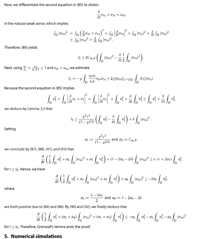
5. Numerical simulations
In this section, we shall present some numerical experiments in order to illustrate the solution behavior in (6). The simulations were carried out using a time-explicit finite difference scheme on an equidistant spatial grid with grid size 0.005 and time step size 10~6. In all diagrams below, the ordinate and abscissa represent the spatial variable x e [0,1] and the time f > 0, respectively. Figure 1 underlines the attractivity result derived for the steady state of (6) in this paper when / is "small" and A is "large! Because we did not derive explicit bounds for the constant Coo(/o»^o) introduced in Corollary 2.8, we do not carry out a precise verification of (84) here. Nevertheless, the steady state seems to be attractive also for this choice of parameters.
Going beyond this, Figure 2 indicates that solutions of (6) still stabilize when neither of our sufficient conditions for the statements in Lemma 3.2 and Theorem 4.1 are satisfied.
Figure 1. Solution behavior for % = 0.1, A = 1, v = 1,u0 = Oand v0 — 1. Vertical axis: x; horizontal axis: t.
Figure 2. Large time behavior for % = 10, A = 1, v = 1,uo = Oand vo(x) = 1 + sin2(2.5?rx).
0 OHHI a.UM (US6 O.Wfl 0.01 0 C H I U K P.MS 1 M B D.Ol
Figure 3. Behavior forO < f < 0.01 for % = 10, A = 1, v = 1,u0 = Oand v0(x) = 1 + sin2(2.5?rx).
Acknowledgements
This work was supported by the visiting professorship program Mercator of the Deutsche Forschungsgemeinschaft within which J.l.Tello visited the University of Duisburg-Essen in autumn 2010. The second author also acknowledges support by project MTM2009-13655 MICINN (Spain). The authors would like to thank Christian Thiel for his valuable assistance concerning the numerical simulations.
References
1. Entchev EV, Schwabedissen A, Gonzalez-Gaitan M. Gradient formation of the TGF/3 homolog Dpp. Cell 2000; 103:981-991. 2. Entchev EV, Gonzalez-Gaitan M. Morphogen gradient formation and vesicular trafficking. Traffic 2002; 3:98-109.
3. Kerszberg M, Wolpert L. Mechanism for positional signalling by morphogen transport: A theoretical study. Journal of Theoretical Biology 1998; 191:103-114.
4. Krzyzanowski P, Laurencot Ph, Wrzosek D. Well-posedness and convergence to the steady state for a model of morphogen transport. SIAMJournal on Mathematical Analysis 2008; 40(5):1725-1749.
5. Krzyzanowski P, Laurencot Ph, Wrzosek D. Mathematical models of receptor-mediated transport of morphogens. Mathematical Models and Methods in Applied Sciences 2010; 20(11):2021-2052.
6. Lander AD, NieQ, Vargas B, Wan FYM. Aggregation of a distributed source morphogen gradient degradation. Studies in Applied Mathematics 2005; 114(4):343-374.
7. Lander AD, Nie Q, Wan FYM. Do morphogen gradients arise by diffusion? Developmental Cell 2002; 2:785-796.
8. Lander AD, Nie Q, Wan FYM. Internalization and end flux in morphogen gradient degradation. Journal ofComputational and Applied Mathematics 2006;190(1-2):232-251.
9. Turing AM. The chemical basis of morphogenesis. Philosophical Transactions of the Royal Society of London 1952; 237:37-72.
11. Merkin JH, Needham DJ, Sleeman BD. A mathematical model for the spread of morphogens with density dependent chemosensitivity. Nonlinearity 2005;18(6):2745-2773.
12. Levine HA, Sleeman BD. A system of reaction-diffusion equations arising in the theory of reinforced random walks. SIAM Journal on Applied Mathematics 1997; 57(3):683-730.
13. OthmerHG, Stevens A. Aggregation, blowup, and collapse: The ABC's of taxis in reinforced random walks. S//A/W Journal on Applied Mathematics 1997; 57(4):1044-1081.
14. Hillen T, Painter K. A user's guide to PDE models for chemotaxis. Journal of Mathematical Biology 2009; 58(1-2):183-217.
15. Winkler M. Global solutions in a fully parabolic chemotaxis system with singular sensitivity. Mathematical Methods in the Applied Sciences 2011; 34(2):176-190.
16. Winkler M. Absence of collapse in a parabolic chemotaxis system with signal-dependent sensitivity. Mathematische Nachrichten 2010; 283(11): 1664-1673.
17. Aida M, Osaki K, Tsujikawa T, Yagi A, Mimura M. Chemotaxis and growth system with singular sensitivity function. Nonlinear Analysis RWA 2005; 6(2):323-336.