Mapping wood production in European forests

Mapping wood production in European forests

Pieter J. Verkerk , Christian Levers , Tobías Kuemmerle , Marcus Lindner , Rubén Valbuena ,

Peter H. Verburg , Sergey Zudin

1. Introduction

Forests provide a broad range of ecosystem services that are important to human society (Millennium Ecosystem Assessment, 2005). Wood production represents a key provisioning service and global wood production amounted to 3.4 billion m3 in the year 2005 (FAO, 2010). Because wood production affects the provision-ing of other services and biodiversity (Schwenk et al., 2012; Verkerk et al., 2014a; Zanchi et al., 2014), spatially explicit infor-mation on wood production is important for the design and imple-mentation of policies targeted at sustainable forest use (cf. Cowling et al., 2008; Maes et al., 2012).

Statistical information on wood production can be combined with land-cover maps (i.e., forest cover maps) to develop wood production maps (Maes et al., 2012). Yet, the use of forest cover as the only proxy to map wood production is a coarse and simplis-tic approach that may result in substantial errors (Eigenbrod et al.,

2010), because production patterns may not be equally distributed across forested landscapes (Wendland et al., 2011; Masek et al., 2011). This suggests that determinants other than forest cover should be considered when mapping wood production patterns.

However, their analysis focussed primarily on understanding dri-vers of harvesting intensity and was restricted to exploring spatial patterns for larger administrative units (national to provincial level or forestry districts) thereby not addressing wood production at the grid level.

Existing studies suggest that knowledge of the factors driving patterns in wood production can improve the disaggregation of wood production statistics substantially. In such an approach first a statistical relationship between a target variable (e.g., wood pro-duction) and its location factors (e.g., soil quality, topography, accessibility) is established at the level of the aggregated target data (e.g., for administrative units). Second, this relationship is then used to predict the suitability of every location for the target variable at the target grid level for which information on the loca-tion factors are available. Such a downscaling approach in which statistical relationships are transferred across scales is called dasy-metric mapping (Eicher and Brewer, 2001) and has been used extensively to disaggregate national- or regional-level land-use extent (Dendoncker et al., 2007), farming systems (van de Steeg et al., 2010), livestock (FAO, 2007; Neumann et al., 2009), or nitro-gen input (Temme and Verburg, 2011). In a forestry context, dasy-metric mapping was used to derive gridded maps of tree species presence for Europe (Brus et al., 2012) and at the global scale to map growing stock, forest biomass (Kindermann et al., 2008) and wood production (Hurtt et al., 2006). The latter maps have been generated at a resolution of Io x Io grid cells, using coarse, national-scale data on wood production, mainly targeted as an input for global climate and vegetation models. These applications strongly highlight the potential for dasymetric mapping to provide insights into wood production patterns, but a fine-scale application of this kind is missing for Europe, and as a result the spatial pat-terns of wood production remain weakly understood.

Here, we present an approach to fill this knowledge gap by developing high-resolution wood production maps for European forests (in this study limited to 27 European Union member states, plus Norway and Switzerland) for the period 2000-2010 at a reso-lution of 1 x 1 km2 grid cells. Our objectives were (1) to analyse the location factors determining wood production patterns in Europe, (2) to assess whether information about the relationship between wood production and location factors improves the disaggregation of wood production statistics, and (3) to derive time series of wood production maps for Europe.

2. Material and methods

2.1. Data

2.1.1. Wood production data

We collected data on wood production from national forestry reports, statistical yearbooks and databases, and by contacting national experts known to the authors (Table SI in the Supplemen-tary Material) for the years 2000 to 2010 for 460 administrative units within the 29 countries in our study. The number of admin-istrative units per country varied from 1 (national level) to 107 (provincial or forestry district level). The statistics that were col-lected followed national definitions and differed in e.g. whether wood production volumes were reported as over or under bark, or included harvest losses. To account for these differences, we harmonised the wood production data by calculating the share of harvested wood volume for each administrative unit relatively to the national total wood production. These shares were calculated as averages for all years for which regional data was available in our dataset. Shares were then multiplied with national-level har-vest data. For the latter, we used annual roundwood production (m3 under bark) statistics from FAOSTAT (2012), because these

data are reported following harmonised definitions and data were available for each year in our study period. To use the data for sta-tistical analyses, we divided harvest volume by forest área in each región (Table S2 in the Supplementary Material). To mitígate prob-lems due to differences in national definitions, we calculated the área share of each unit in the total forest in a particular country and multiplied it with the forest área in 2000 according to Forest Europe et al. (2011). The outcome was a set of maps of harmonised wood production statistics [WOOD; m3 ha- 1 yr- 1] at the level of administrative units.

2.1.2. Location factors

We reviewed literature to identify potential location factors that could affect the likelihood of harvesting at a given location. The literature review focussed on understanding the harvesting behaviour of forest owners (Beach et al., 2005; Bolkesjo et al., 2007; Butler, 2006; Favada et al., 2009; Stordal et al., 2008; Vokoun et al., 2006; Adams et al., 1991; Araño and Munn, 2006), as well as on wood supply in more general terms (Sterba et al., 2000; Verkerk et al., 2011). Based on our review and data availabil-ity for the entire study área, 16 potential location factors influenc-ing the likelihood of harvest were identified, as well as a priori assumptions with regards to the direction of influence of each loca-tion factor on harvesting likelihood (Table 1). This set of potential location factors is similar to the set used by Levers et al. (2014). A key difference is that we used net annual increment as an addi-tional predictor, as it may strongly influence the location of wood production, whereas Levers et al. (2014) used net annual incre-ment to normalise harvest in order to obtain a more direct indica-tor of harvesting intensity at the level of administrative units.

Most data on location factors were available as ráster maps with a resolution of 1 x 1 km2 grid cells. Where data were available at a finer resolution, we aggregated them using bilinear interpolation based on the weighted distance of the four nearest input cell cen-tres. Data layers that were available for administrative units were rasterized to the l x l km2 grid assuming homogeneity across administrative units. Maps of the location factors are shown in Fig. SI in the Supplementary Material. Details on the data pre-processing of the predictor variables are provided in the Supple-mentary Material of Levers et al. (2014).

To match the spatial resolution of our location factors to that of the wood production statistics, we calculated average valúes of our location factors for each of the administrative units for which we had collected wood production statistics. In case location factors were not limited to forests (e.g., P00RS0IL in Table 1), we weighted location factor valúes according to forest cover for each adminis-trative unit. To do so, we multiplied relevant location factor maps with a fractional forest cover map. We used the forest map by Pekkarinen et al. (2009), which was calibrated following an approach by Páivinen et al. (2001) to match regional-and national-level forest área statistics (Section 2.1.1; Table S2 in the Supplementary Material). As a result, the valúes of location factors at locations with higher forest cover had a larger share in the aver-age predictor valué at the administrative unit level, compared to pixels with little forest cover.

We also investigated possible collinearity between location fac-tors, but did not find correlation coefficients exceeded 0.7 (Fig. S2 in the Supplementary Material) and therefore considered all loca-tion factors for subsequent regression analyses.

2.2. Regression analyses

Table 1

Description of location factors used in the regression analyses (cf. Levers et al., 2014). Predictor

Forest resources Extent of forest Growing stock Productivity Tree species composition Protected áreas Abbreviation FCOV2000 TOTVOL NAI BEECHOAK PINESPRUCE PLANTATION TOTPROT Environmental conditions Soil productivity Precipitation Temperature Water shortage Accessibility Accessibility Slope Soil bearing capacity Socio-economy Prívate forests Population density POORSOIL PRCP5M TEMP WATSHORT ACC50 RUCC SBC PRIVFOR POPDENS Description

Forest cover in 2000 Total growing stock

Net annual increment (average over 2000-2010)

Share of beech (Fagus spp.) and oak (Queráis spp.) in total species Share of Scots pine (Pinus sylvestris) and spruce (ñcea spp.) in total species

Share of plantation species (Robinia spp., Populus spp., Eucalyptus spp., Pinus pinaster) in total species

Share of protected forest in total forest

Share of low productive soil limiting growth Precipitation sums of growing season Long term mean temperature

Difference between precipitation and potential evapotranspiration

Travel time to cities > 50,000 inhabitants Terrain ruggedness expressing relief energy Share of soil types with no bearing capacity

Share of forest that is privately owned

Population density (number of people per square kilometre)

Expected impact + + + + + + " -+ + -+ — -+ -Unit %

m3 h a- 1

m3 h a- 1 yr_ 1

% % % % % mm °C mm min m % % pers/km2 Source

Pekkarinen et al. (2009) Gallaun et al. (2010) See Table S3 in the Supplementary Material Brus et al. (2012) Brus et al. (2012)

Brus et al. (2012)

IUCN and UNEP-WCMC (2012) and EEA (2011)

Verkerketal. (2011)

Hijmans et al. (2005) Hijmans et al. (2005) Hijmans et al. (2005)

Nelson (2008)

Riley et al. (1999), Christoph Plutzar (pers. comm.) EC (2006) and Verkerk et al. (2011)

Pulla et al. (2013)

Oak Ridge National Laboratory (2004)

(2) Boosted Regression Trees (BRTs). Algorithmic regression mod-els such as BRTs often outperform traditional, linear regressions in terms of predictive accuracy while being able to model non-linear, complex relationship and being less affected by small sam-ple size and collinearity in input data. However, such non-linear, complex models might be disadvantageous in dasymetric map-ping, because they may result in over- or underestimation when transferring models from the level of administrative units to the grid level. Traditional linear regressions, while potentially less powerful in terms of predictive power, yield regression coefficients that are more robust to scaling between the level of model fitting and prediction (Easterling, 1997; Jelinski and Wu, 1996). Henee, we decided to compare both approaches. For all analyses we used WOOD averaged over our entire study period as the dependent variable, and the location factors as independent variables. We used R (R Development Core Team, 2013) for all statistical analy-ses, including the packages 'dismo' (Hijmans et al., 2013; Boosted regression trees), 'BMA' (Raftery et al., 2013; Bayesian model aver-aging), and 'ráster' (Hijmans, 2014).

2.2.1. Bayesian model averaging

Our first model (hereafter referred to as linear model) was obtained using BMA. We applied BMA to account for uncertainty in the process of model selection, which may lead to over-confident inferences (Hoeting et al., 1999). A single-best model is usually selected among alternative models based on hypothesis tests and goodness-of-fit measures (Raftery et al., 1997). Alterna-tive models that may perform equally well as the "best" model are thus neglected (Hoeting et al., 1999). BMA provides a solution to this by averaging over all possible models to derive a model that accounts for uncertainty in the model selection process and usually yields a better predictive performance compared to a single-best model (Raftery et al., 1997; Madigan and Raftery, 1994).

To carry out the BMA, we used the bicreg function of the BMA package that uses the Bayesian Information Criterion (BIC; Hastie

et al., 2011) to identify the 25 best models of all possible models. We then used the five best candidate models to select the final suite of location factors for the linear model following Raftery et al. (2005). We included only location factors which were consis-tently selected throughout all 25 best models. We furthermore cal-culated the cumulative posterior probability of the five best candidate models to estímate the probability that the "true" model consists of their suite of location factors.

2.2.2. Boosted regression trees

Boosted regression trees are a machine learning technique that combines high predictive accuracy with a good interpretability of results (Friedman, 2001). BRTs are robust against overfitting (Dormann et al., 2013), missing data, and collinearity of location factors, while being able to handle non-linear relationships and variable interactions well (Elith et al., 2008). We fitted two models using BRTs; one with the location factors identified by BMA for the linear model (hereafter referred to as BRTÍ model) and another using the full suite of location factors (hereafter referred to as BRT2 model). We developed these two models to improve the com-parability of results since BRTs selected different variables as most influential in comparison to BMA due to differences in model characteristics.

10-fold cross-validated correlation coefficients. Finally, we set tree complexity to 8 for the BRT1 model (same location factors as in the BMA) and 6 for BRT2 model (all location factors) as well as learning rate to 0.005 and bag fraction to 0.5 for both BRT models.

We employed the gbmstep routine provided by the dismo pack-age to determine the optimal number of trees. To evalúate model performance, we used a 10-fold cross-validation to calcúlate Pear-son's correlation coefficient and the percentage of deviance explained (Elith et al., 2008). For interpreting results of both BRT models, we regarded only those variables as influential which rel-ative importance exceeded that expected by chance (100%/number of variables; i.e. 100%/16 = 6.25%) (Müller et al., 2013). The relative importance thus depends on how often a variable is selected in the models' regression trees and the weighted improvement to the model (Friedman and Meulman, 2003). The sum of all variables' relative importances adds up to 100%, with higher valúes indicat-ing a stronger influence of this particular variable on the target variable (i.e., wood production in our case). To investígate the rela-tionship between each predictor and the target variable, we used partial dependency plots (PDPs) that depict response curves for each location factor along its data range in relation to the wood production while holding all other location factors at their mean (Friedman, 2001).

2.3. Disaggregation and accuracy assessment

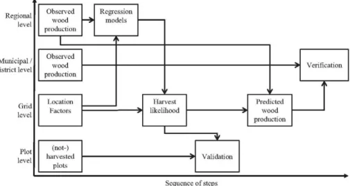
To produce wood production maps, we followed the procedure illustrated in Fig. 1. We first applied the above regression models to produce harvest likelihood maps, and we then used these likeli-hood maps as a basis to disaggregate wood production statistics to the grid level. We developed one likelihood map for each of the three final regression models (linear, BRTÍ, and BRT2, i.e. three harvest likelihood maps in total) by predicting wood production at the l x l km2 grid level and normalising the predictions to valúes between 0 (low likelihood) and 1 (high likelihood) using the mín-imum and máxmín-imum valúes.

We then validated the three likelihood maps using plot data from the 3rd Spanish National Forest Inventory (MAGRAMA, 2013). We used data from a total of 84,264 plots that were located on the Spanish mainland and had a forest cover >20%, of which 224 plots (0.27%) were classified as being recently harvested. We deter-mined the harvest likelihood valué for each of the inventory plots of the linear and the two BRT models. We hypothesised that the recently harvested plots had a larger likelihood score than the unharvested plots and we tested for significance with one-tailed

Mann-Whitney U tests, as data were not normally distributed in all cases.

After generating and validating the harvest likelihood maps, we developed a disaggregation procedure to map wood production at the grid level. To test whether the disaggregation of wood produc-tion statistics is improved by adding informaproduc-tion on locaproduc-tion fac-tors of wood production patterns, we first disaggregated wood production volumes based on forest cover only. The wood produc-tion volume that was allocated to an individual pixel was based on the forest cover of that pixel proportional to the total forest área of all pixels in this administrative unit. Subsequently, we relied on the same disaggregation procedure, but included information from the likelihood maps. We did this by multiplying each harvest like-lihood map with the forest cover map. As a result, the wood pro-duction volume that was allocated to an individual pixel was larger for pixels with higher harvest likelihood and higher forest cover valúes, compared to pixels with e.g. higher harvest likeli-hood, but lower forest cover valúes.

We verified our disaggregation results following Neumann et al. (2009) and re-aggregated grid-level wood production to the level of finer administrative units than those used for building the regres-sion models and for which independent data was available. We ver-ified our disaggregation results for 44 districts in Baden-Württemberg (Germany) and for 410 municipalities in Norway. We used Spearman correlation tests to test how well our predictions matched with observed wood production levéis. To avoid inflating correlation coefficients we excluded countries for which we had only data at the national level. Furthermore, we calculated differ-ence maps between predicted wood production (based on the disag-gregation of national level statistics) and observed wood production at the level of administrative units. Based on this accuracy assess-ment, we selected the likelihood map that resembled observed wood production statistics best and produced a final European-wide wood production map. We used R (R Development Core Team, 2013) for all statistical analyses, including the 'rgdal' (Bivand et al., 2013) and 'ráster' (Hijmans, 2014) packages.

3. Results

3.1. Regression results

The cumulative posterior probability of the top five BMA mod-els was 0.79, indicating a high probability that the "true" model consists of location factors selected by these models. Six location factors were selected based on their posterior probabilities of

Regional level

Municipal / district level

Grid level

Plot level

Observed wood production

1

wood production

Location Factors

Regression

> v

> f Harvest

> '

Predicted prodi LCtion

Verifícation

t _\

(not-) harvested

plots

Validation

Sequence of steps

Table 2

Results of the linear model. The abbreviations of the location factors are explained in Table 1.

Coefficient a b c d e f g

Intercept POORSOIL PRCP5M RUGG PLANTATION PINESPRUCE NAI

Estímate -1.181* - 0 . 0 2 1 "

0.006" - 0 . 0 1 3 " 0.056" 0.021" 0 . 3 3 1 "

SE 0.369 0.006 0.001 0.002 0.010 0.004 0.047 Significance levéis: "p < 0.01; "p < 0.001.

inclusión: POORSOIL, PRCP5M, RUGG, PLANTATION, PINESPRUCE and NAL These variables were consistently selected in each of the top five models. We used these six location factors in the final linear model with wood production averaged over the entire 11 -year per-iod as the dependent variable (WOOD). The final linear model was expressed as follows:

WOOD = a + bPOORSOIL + CPRCP5M + dRUGG + ePLANTATION +fPINESPRUCE + gNAI

in which coefficients a-g are the regression parameters. The results of the regression analysis for the linear model are presented in Table 2. The linear model was highly significant (p < 0.005) and explained (adjusted R2) about 45% of the variance in wood

produc-tion patterns. All locaproduc-tion factors confirmed our a priori assump-tions with regards to the direction of their influence (positive or negative; see also Table 1) on wood production. NAI revealed the strongest absolute effect on wood production.

The same set of six location factors was used in the BRTl model (Fig. 2) and explained about 67% of the variance in wood produc-tion patterns. Similar to the linear model, NAI was the most impor-tant variable for explaining the spatial patterns in wood production with a relative importance of about 30%, whereas PLANTATION was the second-most important predictor with a relative importance of about 26%. All location factors had the same, expected sign as for the linear model. However, the boosted regression trees revealed that not all location factors were linearly related to wood produc-tion at the administrative level. In case of PLANTATION, for exam-ple, wood production was found to decrease below a threshold of 20% plantation species in total forest cover, after which it increased and saturated at a threshold of 40% plantation species.

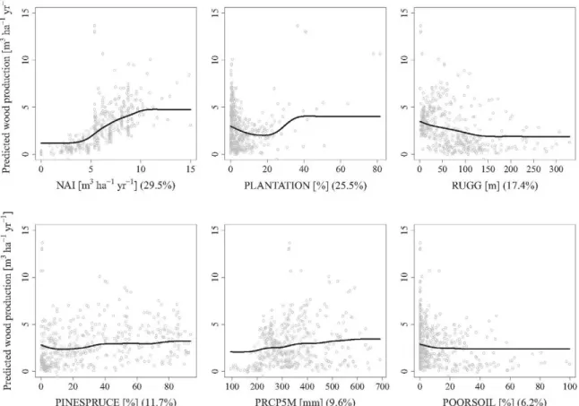
The BRT2 model (Fig. 3) performed slightly better than the BRTl model, explaining about 71% of the variance in wood production patterns. The location factors NAI, PLANTATION, RUGG, ACC50, and TOTVOL were most influential. Similar to the other models, NAI was the most important variable (24%) for explaining the spatial patterns in wood production and PLANTATION (18%) was the second-most important predictor. Compared to the other models, POORSOIL, PRCP5M were less important in the BRT2 model. Instead, ACC50, RUGG and TOTVOL were found to be influential. Similar to the BRTl model, the BRT2 model revealed that not all location fac-tors were linearly related to wood production at the level of administrative units.

3.2. Accuracy assessment

We applied the regression models to produce three harvest like-lihood maps, one for each regression model (Fig. S3 in the Supple-mentary Material). Utilising the Spanish forest inventory plot data,

NAI [m3 ha"1 yr"1] (29.5%)

0 20 40 60 80

PLANTATION [%] (25.5%)

0 50 100 150 200 250 300

RUGG [m] (17.4%)

0 20 40 60 80

PINESPRUCE [%] (11.7%)

100 200 300 400 500 600

PRCP5M [mm] (9.6%)

700 20 40 60 80 100

POORSOIL [%] (6.2%)

5 10 15 NAI [m3 ha"1 yr"1] (24.4%)

0 20 40 60 80 PLANTATION [%] (18.2%)

0 50 100 150 200 250 300 RUGG [m] (9.4%)

200 400 600 800 ACC50[min](8.1%)

1000 50 100 150 200 250 300

TOTVOL [m3 ha"1] (7.1%)

Fig. 3. Partial dependency plots for the BRT2 model. The y-axis [unit: m3 ha ' yr ' ] of each plot shows the fitted valúes for each observation along the variable's data range

displayed on the x-axis. The ticks on the x-axis visualise the distribution of the data in deciles. The unit of each predictor is described in Table 1.

we tested whether recently harvested plots had a larger harvest likelihood score compared to unharvested plots. The results of three one-tailed Mann-Whitney U tests showed that recently har-vested plots had significantly (p < 0.005) higher likelihood seo res as compared to unharvested plots for all three likelihood maps (Table 3).

Using the forest cover map, as well as the three harvest likeli-hood map, we disaggregated wood production statistics to the grid level. To verify the resulting wood production maps we re-aggregated from the grid-level to the level of finer administrative units and compared the predicted wood production with observed data at the level of administrative units using fine-scale harvesting statistics for Europe, Baden-Wuerttemberg and Norway. Results of Spearman correlation tests (Figs. 4 and 5) between predicted and observed wood production revealed that disaggregating based on forest cover solely yielded the poorest results. When considering additional information (compared to forest cover only), the corre-lation between predicted and observed wood production improved substantially. Between the three regression-based likelihood maps, we observed only minor differences. The disaggregation based on the linear model showed slightly higher correlations compared to the disaggregations based on the two BRT models.

Fig. 6 provides information on the spatial patterns in the differ-ence between predicted and observed levéis of wood production in Europe. When considering forest cover only, wood production was overestimated in North Finland and Sweden, North-West Germany and South-East France, whereas wood production was underesti-mated in South Finland and Sweden, South-West of France, North-West of Spain and Southern parts of Germany. When com-bining forest cover with information derived from the linear and both BRT models, the absolute differences between predicted and

observed data became smaller, but the spatial patterns in the dif-ferences between predicted and observed wood production remained similar.

3.3. Maps of wood production in European forests

Based on the verification described above, we used forest cover combined with information derived from the linear model to dis-aggregate statistics from administrative units to 1 x 1 km2 grid maps. Considering location factors to disaggregate wood produc-tion statistics resulted in a greater variance in wood producproduc-tion at the grid-level, as compared to considering forest cover only (one-tailed F-test, p< 0.005). At the European level, our maps (Figs. 7 and S4) reveal regions with very low levéis of wood pro-duction (<0.1 m3 h a ^ y r "1) , notably the coastal área of Norway, large parts of England, Spain, and Greece as well as northern and eastern Italy and the western parts of Netherlands and Belgium. Regions with high average levéis of wood production (>5 m3 ha"1 yr"1) can be found in southern Sweden, southeast Belgium, northeast France, southern Germany and large parts of the Czech Republic, Austria and Switzerland and northwestern Spain. Average harvest levéis exceeded >10 m3 ha"1 yr"1 in southwestern France.

Table 3

Median likelihood score of three likelihood maps for harvested (n = 224) and unharvested (n = 84,040) Spanish forest inventory plots and the signiflcance levéis according to one-tailed Mann-Whitney U tests.

Coverage Linear model BRT1 model BRT2 model 4. Discussion Harvested 0.38 0.23 0.21 Unharvested 0.20 0.09 0.09 p-Value <0.001 <0.001 <0.001

4.1. Locatíon factors determining spatíal patterns ofwood production Wood production is an important forest use and understanding the spatial patterns of harvesting is key for assessing how it might affect ecosystem services and biodiversity. Yet, wood production statistics are often only available for larger administrative units, requiring downscaling to assess the spatial patterns of harvesting. In this study we developed high-resolution wood production maps of European forests. We analysed the location factors of spatial pat-terns in wood production across a forest área of more than 163 million ha in Europe and found that increment, tree species com-position, and terrain ruggedness were key location factors explain-ing patterns in wood production in Europe between 2000 and 2010. Other important location factors that we identified were growing stock volume, accessibility, precipitation amounts, as well as soil productivity. As such, our analysis of location factors that influence spatial patterns in wood production is in broad

agreement with those reported by Levers et al. (2014), despite their focus on harvesting intensity (i.e., wood production in relation to the net annual increment) rather than wood production.

The identified location factors all relate to the costs and prof-itability of wood production, as harvest likelihood is higher under more productive growing conditions and in locations that can be more easily harvested. Our findings thus provide important infor-mation to further improve existing estimates of the costs of wood supply (cf. de Wit and Faaij, 2010; Lauri et al., 2014). While there is a potential to increase wood or biomass production in Europe to meet future material and energy demands (Verkerk et al., 2011), it is not clear where such unutilised potentials are located. Based on our set of location factors that determine current wood produc-tion patterns, unutilised potentials are likely located in áreas that have lower increment rates (resulting in lower harvest volumes or longer production cycles) and are more remote or rugged. This implies that the costs to mobilise these unutilised potentials could be higher compared to the costs for current wood production.

4.2. Spatial patterns of wood production

We disaggregated wood production statistics from the level of administrative units to ráster maps with a resolution of l x l km2. We show that forest cover alone is a poor proxy to map wood production, as wood production is not equally dis-tributed across European forest landscapes. When considering for-est cover only, we would underfor-estimate wood production in productive, accessible regions and overestimate production in less productive and less accessible regions. When we included our

20000 15000 10000 5000 0 -Forest cover

Correlation = 0.882 /

O /

o /

°° /

2S&3 ° °

\ l i l i

Forest cover & GLM model

20000 _Correlation

15000 Foi 20000 15000 10000 5000 0

-est cover &

Correlation

O / Q5 /

/SgRbo

mSo o

B K 1 1 m o = 0.95 /

0 / Foi 20000 15000 10000 5000 0

-est cover &

Correlation

O /

00

/

M o o

T 1 1 B K 1 2 m o = 0.95 /

o / 1 1 600 500 400 300 200 100 0

-Correlation = 0.959 °/

o

X

6/

T 1 1 1 1 1 1

600 500 400 300 200 100 0

-Correlation = 0.96? /

tf/o

áSSÍO

T 1 1 1 1 1 1

600 500 400 300 200 100 0

-Correlation = 0.964° /

$A

dÉÜrP

T 1 1 1 1 1 1

"E

í

°°<h

o

y

oflBP o

r i i i

0.883 /

/ o

0 0

1 1 1

300 250 200 150 100 50 0

-Correlation = 0.918

O

T ^

8 o - /

o o / o

K8BS °

(o? O

1 1 1 1 1

O 1 300 250 200 150 100 50 0

-Correlation = 0.905 /

oí

° ° o / o

o /$

«B ° Po

W

300 250 200 150 100 50 0

-Correlation = 0.902 /

° ° o / o

o

y

mtk°°

Forest cover Forest cover & GLM model

10-£ -¿ C

15-

10-Forest cover & BRT1 model

15-

10-Forest cover & BRT2 model

15-

10-Forest cover Forest cover & GLM model Forest cover & BRT1 model Forest cover & BRT2 model

10-

15-

10-

15-

10-

15-

10-Forest cover

15-

105

-o -o-l,

Predicted (m3 ha ' yr ')

Forest cover & GLM model

1 5

-

105

-0-1

Predicted (m ha yr )

Forest cover & BRT1 model

1 5

1 0

5

-0 4

Predicted (m3 ha ' yr ')

Forest cover & BRT2 model

1 5

1 0

5

-0-1

Predicted (m ha yr )

Fig. 5. Results of Spearman correlation tests between observed and predicted wood production per unit of forest área [unit: m3 ha-1 yr-1 ] based on disaggregating statistics using four different likelihood maps for Europe (from 19 countries to 451 administrative units; top row), Baden-Württemberg (from 1 state to 44 districts; middle row) and Norway (from 19 provinces to 410 municipalities; bottom row).

Forest cover Forest cover & linear model Forest cover & BRT1 model Forest cover & BRT2 model

m

i

WA

gTM

.í

«

i-víS»

_%

<-10.0 -9.9 - -5.0 -4.9--1.0 -0.9 - 1.0 1.1 -5.0 5.1 -10.0 > 10.0

Fig. 6. Maps showing the difference between predicted and observed wood production [unit: m3 ha ' forest yr '] in Europe based on four different maps to disaggregate national-level statistical data.

harvest likelihood maps, the differences between predicted and observed wood production became smaller. For example, incre-ment and soil productivity differences between regions (Fig. SI in the Supplementary Material) explained the differences between predicted and observed wood production in Finland, Germany and Sweden, with northern regions in these countries generally having lower increment rates as compared to southern regions. In Finland, northern regions also had larger áreas with less productive soils. In

France and Spain plantation species (Fig. SI in the Supplementary Material) explain why wood production was larger than average in southwest France and northwest Spain as compared to other regions in these countries.

0'0"W

T

20°0'0"W 10°0'0"W 0°0'0" 10°0'0"E 20°0'0"E 30°0'0"E 40°0'0"E

Fig. 7. Map showing predicted wood production [unit: m3 ha ' land yr units to 1 x 1 km2 ráster maps with the linear model.

| in Europe averaged over the period 2000-2010 by disaggregating statistics from administrative

statistical data only. We found that incorporating location factors in our disaggregation resulted in a greater variance in wood pro-duction at the grid-level, as compared to considering forest cover only. Because the provisioning of various ecosystem services is affected by wood production (Schwenk et al., 2012; Verkerk et al., 2014a; Zanchi et al., 2014), our maps therefore provide improved information on how other ecosystem services are affected by local differences in wood production.

Our time-series of wood production maps revealed few, but rel-atively large changes in wood production volumes locally (Figs. S4 and S5 in the Supplementary Material). For most of the cases, these large changes are likely the result of salvage harvest following big storm events. Locally, storm Lothar (December 1999; effect visible in 2000) affected southern Germany, northeast France and Switzerland, storm Gudrun (January 2005) affected southern Sweden, storm Kyrill (January 2007) affected especially central Germany, and storm Klaus (January 2009) affected southwest France (Gardiner et al., 2010). Our maps indícate the approximate location impacted by these storms (as well as other, less damaging storms) and thus allow to estímate changes in wood harvesting (and ecosystem service portfolios) associated with such storm events. Including data on storm tracks when generating harvest likelihood maps could be an interesting avenue for future research to better account fo the effects of salvage harvests.

4.3. Comparison of regression models

techniques may be more appropriate for dasymetric mapping, when statistical relationships are used to disaggregate statistics at finer resolutions.

4.4. Uncertainties in wood production maps

We mapped wood production based on official statistics. It is important to note that such statistics do not necessarily include all wood that is removed from forests. Trees may be harvested to produce firewood for own consumption and such wood remováis may not be recorded in official statistics (Steierer, 2010). This means that the mapped wood may be an underestimation.

Based on a literature review we identified a number of location factors that are associated with the spatial patterns in wood pro-duction. Only few of these location factors significantly explained wood production patterns. The share of protected forests was not found to affect wood production patterns, although it has been linked to a potential reduction in wood supply (Verkerk et al., 2014b). We explain such apparent discrepancies by gaps in avail-able data. In the case of protected forests, we used spatially explicit data from two databases (IUCN and UNEP-WCMC, 2012; EEA, 2011). However, these dataseis do not include all existing pro-tected forests (Mac Sharry, 2011), ñor do they contain detailed information on restrictions applied to wood production. This means that although we did not find a predictor to significantly affect wood production in our regression analyses, it may still be a factor of relevance.

Likewise, some predictors we would have wished to include were not available in a consistent, spatially-explicit manner for the whole study área. An important factor that could help to explain the spatial patterns of wood production, but which was not considered here, relates to the location of and distance to wood processing facilities, including pulp- and sawmill and energy pro-duction facilities that use wood as a feedstock. We expect that higher levéis of wood production could be observed closer to such facilities and production sites.

Our approach may have excluded local location factors that determine spatial variability in wood production across land-scapes. The analysis of location factors at the level of larger admin-istrative units can only partly account for factors that determine variations at the local to landscape level, e.g. environmental factors such as soil conditions, or socio-economic factors such as owner-ship. Despite these remaining uncertainties, our set of location fac-tors explained a substantial part of the spatial variation in wood production and resulted in a robust disaggregation of wood pro-duction statistics, as verified by our comparison to the municipal level. The results of our validation of the regression-based likeli-hood maps do suggest that our wood production maps are well able to capture local patterns of wood production. However, while the accuracy assessment steps we carried out suggest our approach resulted in reliable wood production maps, we caution that we only had validation and verification data for some regions, from the Mediterranean to Scandinavia. A consistent and spatially detailed ground-based dataset on wood production is not readily available for Europe currently. We can thus not rule out the possi-bility that our map is less reliable in áreas where we did not have such data. A harmonised, European-wide datábase with data from national forest inventories would be an invaluable data source for a future, more in-depth accuracy assessment.

5. Conclusión

We conclude that several location factors are important in explaining variation in wood production patterns across Europe: productivity, tree species composition and terrain ruggedness.

Other important factors are growing stock volume, accessibility, precipitation amounts and site productivity. Incorporating such information significantly improves the disaggregation of wood production statistics from the regional level to the grid level as compared to disaggregation based on forest cover maps only. The final wood production maps give insight into forest ecosystem ser-vice provisioning and can be used to improve the assessment of potential and costs of woody biomass supply.

Acknowledgements

The authors thank Anze Japelj and Rok Pisek for providing data on regional wood production for Slovenia, Elena Rafailova for pro-viding data on regional wood production for Bulgaria, Katja Gunia for providing statistics on forest área and net annual increment, Christoph Plutzar for providing data on terrain ruggedness and Mart-Jan Schelhaas and Geerten Hengeveld for comments on the methods. This work has been funded through the EU 7th frame-work projects VOLANTE and GHG-Europe (project numbers 265104 and 244122). Tobias Kuemmerle acknowledges funding by the Einstein Foundation Berlin, Germany. Opinions expressed in this paper are those of the authors only.

References

Adams, D.M., Binkley, C.S., Cardellichio, P.A., 1991. Is the level of national forest timber harvest sensitive to price? Land Econ. 67 (1), 74-84.

Araño, K.G., Munn, I.A., 2006. Evaluating forest management intensity: a comparison among major forest landowner types. For. Policy Econ. 9, 237-248. Beach, R.H., Pattanayak, S.K., Yang, J.-C, Murray, B.C., Abt, R.C., 2005. Econometric studies of non-industrial prívate forest management: a review and synthesis. For. Policy Econ. 7, 261-281.

Bivand, R., Keitt, T., Rowlingson, B., Pebesma, E., Sumner, M., Hijmans, R., Rouault, E., 2013. rgdal: Bindings for the Geospatial Data Abstraction Library. <http://cran.

r-project.org/web/packages/rgdal> (19.12.14).

Bolkesjo, T.F., Solberg, B., Wangen, K.R., 2007. Heterogeneity in nonindustrial prívate roundwood supply: lessons from a large panel of forest owners. J. For. Econ. 13, 7-28.

Brus, D.J., Hengeveld, G.M., Walvoort, D.J.J., Goedhart, P.W., Heidema, A.H., Nabuurs, G.J., Gunia, K., 2012. Statistical mapping of tree species over Europe. Eur. J. Forest Res. 131,145-157.

Butler, B.J., 2006. The Timber Harvesting Behavior of Family Forest Owners. Dissertation. Oregon State University. 130 pp.

Cowling, R.M., Egoh, B., Knight, A.T., O'Farrell, P.J., Reyers, B., Rouget, M., Roux, D.J., Welz, A., Wilhelm-Rechman, A., 2008. An operational model for mainstreaming ecosystem services for implementation. Proc. Nati. Acad. Sci. 105, 9483-9488. de Wit, M, Faaij, A, 2010. European biomass resource potential and costs. Biomass

Bioenergy 34,188-202.

Dendoncker, N., Bogaert, P., Rounsevell, M., Koomen, E., Stillwell, J., Bakema, A., Scholten, H.J., 2007. Empirically Derived Probability Maps to Downscale Aggregated Land-Use Data Modelling Land-Use Change. Springer, Netherlands, pp. 117-132.

Dormann, C.F., Elith, J., Bacher, S., Buchmann, C, Cari, G., Carré, G., Márquez, J.RG., Gruber, B., Lafourcade, B., Leitao, P.J., Münkemüller, T., McClean, C, Osborne, P. E., Reineking, B., Schroder, B., Skidmore, A.K., Zurell, D., Lautenbach, S., 2013. Collinearity: a review of methods to deal with it and a simulation study evaluating their performance. Ecography 36 (2013), 027-046.

Easterling, W.E., 1997. Why regional studies are needed in the development of full-scale integrated assessment modelling of global change processes. Glob. Environ. Change 7, 337-356.

EC, 2006. European Soil Datábase v. 2.0. European Commission - DG Joint Research Centre, Ispra, Italy. <http://eusoils.jrc.ec.europa.eu/ESDB_Archive/ESDB>

(accessed 10.10.12).

EEA, 2011. Nationally designated áreas (National - CDDA). European Environment Agency, Copenhagen. <http://www.eea.europa.eu/data-and-maps/data/ds_

resolveuid/lec5cbd6ab3294e2e7fe6558cd81b940> (accessed 22.03.12).

Eigenbrod, F., Armsworth, P.R., Anderson, B.J., Heinemeyer, A, Gillings, S., Roy, D.B., Thomas, C.D., Gastón, K.J., 2010. The impact of proxy-based methods on mapping the distribution of ecosystem services. J. Appl. Ecol. 47, 377-385. Elith, J., Leathwick, J.R., Hastie, T., 2008. A working guide to boosted regression trees.

J. Anim. Ecol. 77, 802-813.

FAO, 2007. Gridded livestock of the world 2007. Food and Agriculture Organization of the United Nations, Rome, p. 131

FAO, 2010. Global forest resources assessment 2010. FAO forestry paper 163. Food and Agricultural Organization of the United Nations, Rome, p. 340..

FAOSTAT, 2012. Roundwood Production Quantity. <http://faostat.fao.org/site/626/

DesktopDefault.aspx?PageID=626> (accessed 24.1.12).

Favada, I.M., Karppinen, H., Kuuluvainen, J., Mikkola, J., Stavness, C, 2009. Effects of timber prices, ownership objectives, and owner characteristics on timber supply. For. Sci. 55, 512-523.

Forest Europe, UNECE, FAO, 2011. State of Europe's forests 2011. Status and trends in sustainable forest management in Europe. In: Ministerial Conference on the Protection of Forests in Europe. Forest Europe liaison unit Oslo, Aas, p. 337. Friedman, J.H., 2001. Greedy function approximation: a gradient boosting machine.

Ann. Stat. 29, 1189-1232.

Friedman, J.H., Meulman, J.J., 2003. Múltiple additive regression trees with application in epidemiology. Stat. Med. 22,1365-1381.

Gallaun, H., Zanchi, G., Nabuurs, G.-J., Hengeveld, G., Schardt, M., Verkerk, P.J., 2010. EU-wide maps of growing stock and above-ground biomass in forests based on remote sensing and field measurements. For. Ecol. Manage. 260, 252-261. Gardiner, B., Blennow, K., Carnus, J.-M., Fleischer, P., Ingemarson, F., Landmann, G.,

et al., 2010. Destructive storms in European forests: past and forthcoming impacts. Final report to European Commission - DG Environment. European Forest Institute, Atlantic European Regional Office - EF1ATLANTIC, Bordeaux. Hastie, T., Tibshirani, R, Friedman, J.H., 2011. The Elements of Statistical Learning:

Data Mining, Inference, and Prediction. Springer-Verlag, New York, p. 744. Hengeveld, G.M., Nabuurs, G.-J., Didion, M., van den Wyngaert, I., Clerkx, A.P.P.M.,

Schelhaas, M.-J., 2012. A forest management map of European forests. Ecol. Soc. 17.

Hijmans, R.J., 2014. Ráster: Geographic data analysis and modeling. <http://cran.r

-project.org/web/packages/raster> (19.12.14).

Hijmans, R.J., Cameron, S.E., Parra, J.L, Jones, P.G., Jarvis, A., 2005. Very high resolution interpolated climate surfaces for global land áreas. Int. J. Climatol. 25, 1965-1978.

Hijmans, R.J., Phillips, S., Leathwick, J.R. Elith, J., 2013. dismo: Species distribution modeling. <http://cran.r-project.org/web/packages/dismo/> (02.04.13). Hoeting, J.A., Madigan, D., Raftery, A.E., Volinsky, C.T., 1999. Bayesian model

averaging: a tutorial. Stat. Sci. 14, 382-401.

Hurtt, G.C., Frolking, S., Fearon, M.G., Moore, B., Shevliakova, E., Malyshev, S., Pacala, S.W., Houghton, R.A., 2006. The underpinnings of land-use history: three centuries of global gridded land-use transitions, wood-harvest activity, and resulting secondary lands. Glob. Change Biol. 12, 1208-1229.

IUCN & UNEP-WCMC, 2012. The World Datábase on Protected Áreas (WDPA). UNEP-WCMC, Cambridge, UK. <http://www.protectedplanet.net> (accessed 01.02.12).

Jelinski, D., Wu, J., 1996. The modifiable areal unit problem and implications for landscape ecology. Landscape Ecol. 11,129-140.

Kindermann, G.E., McCallum, I., Fritz, S., Obersteiner, M., 2008. A global forest growing stock, biomass and carbón map based on FAO statistics. Silva Fennica 42, 387-396.

Lauri, P., Havlík, P., Kindermann, G., Forsell, N., Bottcher, H., Obersteiner, M., 2014. Woody biomass energy potential in 2050. Energy Policy 6 6 , 1 9 - 3 1 .

Levers, C, Verkerk, P.J., Müller, D., Verburg, P.H., Butsic, V., Leitao, P.J., Lindner, M., Kuemmerle, T., 2014. Drivers of forest harvesting intensity patterns in Europe. For. Ecol. Manage. 315,160-172.

Mac Sharry, B. 2011 Merged European CDDA dataset for 2011. Public versión. European Topic Centre on Biological Diversity (ETC/BD).

Madigan, D., Raftery, A.E., 1994. Model selection and accounting for model uncertainty in graphical models using Occam's window. J. Am. Stat. Assoc. 89, 1535-1546.

Maes, J., Egoh, B., Willemen, L., Liquete, C, Vihervaara, P., Schagner, J.P., Grizzetti, B., Drakou, E.G., Notte, A.L, Zulian, G., Bouraoui, F., Luisa Paracchini, M., Braat, L, Bidoglio, G., 2012. Mapping ecosystem services for policy support and decisión making in the European Union. Ecosyst. Serv. 1, 31-39.

MAGRAMA 2013. Tercer Inventario Forestal Nacional IFN3. <http://www. magrama.gob.es/es/biodiversidad/servicios/banco-datos-naturaleza/informacion-disponible/ifn3_bbdd_descargas.htm.aspx> (05.02.13).

Masek, J.G., Cohén, W.B., Leckie, D., Wulder, M.A., Vargas, R., De Jong, B., et al., 2011. Recent rates of forest harvest and conversión in North America. J. Geophys. Res., G: Biogeosciences 116.

Millennium Ecosystem Assessment, 2005. Ecosystems and Human Well-being: Current State & Trends Assessment, vol. 1, Island Press, Washington. Müller, D., Leitao, P.J., Sikor, T., 2013. Comparing the determinants of cropland

abandonment in Albania and Romanía using boosted regression trees. Agrie. Syst. 117,66-77.

Nelson, A., 2008. Estimated travel time to the nearest city of 50,000 or more people in year 2000. Ispra, Italy: Global Environment Monitoring Unit - Joint Research Centre of the European Commission. <http://bioval.jrc.ec.europa.eu/products/

gam/index.htm> (13.07.11).

Neumann, K., Elbersen, B.S., Verburg, P.H., Staritsky, L, Perez-Soba, M., de Vries, W., Rienks, W.A, 2009. Modelling the spatial distribution of livestock in Europe. Landscape Ecol. 24,1207-1222.

Oak Ridge National Laboratory, 2004. LandScan 2004™ High Resolution global Population Data Set.

Paivinen, R, Lehikoinen, M., Schuck, A., Hame, T., Vaatainen, S., Kennedy, P., Folving, S., 2001. Combining earth observation data and forest statistics. Research Report 14. European Forest Institute and Joint Research Centre/European Commission, Joensuu.

Pekkarinen, A., Reithmaier, L, Strobl, P., 2009. Pan-European forest/non-forest mapping with Landsat ETM+ and CORINE Land Cover 2000 data. ISPRS J. Photogram. Rem. Sens. 64,171-183.

Pulla, P., Schuck, A., Verkerk, P. J., Lasserre, B., Marchetti, M. & Creen, T. 2013. Mapping the distribution of forest ownership in Europe. EFI Technical Report 88. European Forest Institute, Joensuu.

R Core Team 2013. R: A language and environment for statistical computing. R Foundation for Statistical Computing, Vienna, Austria.

Raftery, A.E., Hoeting, J.A., Volinsky, C.T., Painter, L, Yeung, K.Y., 2013. BMA: Bayesian Model Averaging. <http://cran.r-project.org/web/packages/BMA> (02.04.13).

Raftery, A.E., Madigan, D., Hoeting, J.A., 1997. Bayesian model averaging for linear regression models. J. Am. Stat. Assoc. 9 2 , 1 7 9 - 1 9 1 .

Raftery, A.E., Painter, I.S., Volinsky, C.T., 2005. BMA: an R package for Bayesian Model Averaging. R news 5, 2-8.

Riley, S.J., Degloria, S.D., Elliott, R., 1999. A terrain ruggedness Índex that quantifies topographic heterogeneity. Intermount. J. Sci. 5, 23-27.

Schwenk, W.S., Donovan, T.M., Keeton, W.S., Nunery, J.S., 2012. Carbón storage, timber production, and biodiversity: comparing ecosystem services with multi-criteria decisión analysis. Ecol. Appl. 22,1612-1627.

van de Steeg, J.A., Verburg, P.H., Baltenweck, L, Staal, S.J., 2010. Characterization of the spatial distribution of farming systems in the Kenyan Highlands. Appl. Geograph. 30, 239-253.

Steierer, F., 2010. EU/EFTA Sub-regional and National Wood Resource Balances 2005. Geneva Timber and Forest Study Paper 51. UNECE/FAO, Geneva. Sterba, H., Golser, M., Moser, M., Schadauer, K., 2000. A timber harvesting model for

Austria. Comput. Electron. Agri. 28,133-149.

Stordal, S., Lien, G., Baardsen, S., 2008. Analyzing determinants of forest owners' decision-making using a sample selection framework. J. For. Econ. 14,159-176. Temme, A.J.A.M., Verburg, P.H., 2011. Mapping and modelling of changes in

agricultural intensity in Europe. Agrie. Ecosyst. Environ. 140, 46-56. Verkerk, P., Zanchi, G., Lindner, M., 2014b. Trade-offs between forest protection and

wood supply in Europe. Environ. Manage. 53,1085-1094.

Verkerk, P.J., Anttila, P., Eggers, J., Lindner, M., Asikainen, A., 2011. The realisable potential supply of woody biomass from forests in the European Union. For. Ecol. Manage. 261, 2007-2015.

Verkerk, P.J., Mavsar, R, Giergiczny, M., Lindner, M., Edwards, D., Schelhaas, M.J., 2014a. Assessing impacts of intensified biomass production and biodiversity protection on ecosystem services provided by European forests. Ecosyst. Serv. 9, 155-165.

Vokoun, M., Amacher, G.S., Wear, D.N., 2006. Scale of harvesting by non-industrial prívate forest landowners. J. For. Econ. 11, 223-244.

Wendland, K.J., Lewis, D.J., Alix-Garcia, J., Ozdogan, M., Baumann, M., Radeloff, V.C, 2011. Regional- and district-level drivers of timber harvesting in European Russia after the collapse of the Soviet Union. Glob. Environ. Change 21, 1290-1300.