Determinants of demand for natural gas and liquefied natural gas: a country study

Texto completo

(1)DETERMINANTS OF DEMAND FOR NATURAL GAS AND LIQUEFIED NATURAL GAS A COUNTRY STUDY. Abstract In this paper, the determinants of demand for natural gas and for liquefied natural gas (LNG) have been analysed using gravity equations. Two different equations have been developed, one for the total natural gas market and another one for the liquefied natural gas market. For each model, three contrasts have been applied in order to obtain the best possible estimates and to compare between them. The results show a great influence of distance over the trade of natural gas, in both the total and the liquefied market, reducing the quantity traded as the distance is longer. Also, in the LNG market, we can see that countries with a storage capacity over the median import significantly more LNG than the others, showing the importance of those adapted facilities. In addition, it could be said that Europe still depends on pipeline imports, because its weight in world LNG market is low.. Author: SERRANO CATALÁN, VÍCTOR [email protected] Degree in Economics – Group A – Course 2015/2016 Tutor: SUÁREZ BURGUET, CELESTINO JEL Classification: F10, F14, Q02, Q37, Q40, Q41.

(2) Index Introduction……………………………………………………………………………………..4 Reference framework………………………………………………………………………….6 Literature review………………………………………………………………………………13 The model…………………………………………….……………………………………….17 Data…………………………………………………………………………………………….21 Econometrics………………………………………………………………………………….25 Results…………………………………………………………………………………………26 Conclusions……………………………………………………………………………………31 References…………………………………………………………………………………….33 Annexes………………………………………………….…………………………………….37. 2.

(3) Index of figures Figure 1. Main net importers of natural gas, 2014………………………………………….6. Figure 2. World natural gas trade flows, 2014………………………………………………8. Figure 3. Regasification capacity by country, 2012-2017………………………………...10. Figure 4. Results of the regressions made with the total natural gas market model….26. Figure 5. Results of the models applied to study the LNG market………………………28. 3.

(4) DETERMINANTS OF DEMAND FOR NATURAL GAS AND LIQUEFIED NATURAL GAS. A COUNTRY STUDY Introduction The aim of the present paper is to study the determinants of demand for natural gas and also for liquefied natural gas (LNG), by using gravity equations to analyse the main transportation costs of this fuel and the factors that make its trade easier. The relevance of this topic comes from the growth that this fuel is experiencing during last years, thanks to the fact that, when it is burned, it emits less CO 2 to the atmosphere than oil or coal. This characteristic makes it interesting for developing countries with a great industrial sector, like China, because it helps to reduce pollution, and those countries can fulfil their international agreements in terms of emissions reduction without affecting their industrial sector (Schaffer, 2008). Furthermore, in the trade of this product, which has a capital-intensive supply chain, the advance of technology during the last decades has played a key role, mainly for the liquefied natural gas. LNG needs to be transported in special ships, known as methane ships or tankers, and also some adapted facilities to liquefy and regasify it, as we will see below. Those infrastructures have been benefited from the advance of technology, which has improved their storage capacity and their efficiency (Maxwell and Zhu, 2011). This is not the only factor that explains the importance of the natural gas nowadays. As Nick and Thoenes (2014) appointed, the study of this fuel is important because it is used in many different areas, from the industrial production to residential use for heating, and more recently as a fuel for ecological vehicles. Kumar et al. (2011) predict that natural gas consumption will continue growing in the following years. In the present study, the factors that mainly affect the natural gas trade (and that appear in most of the literature about gravity models), like the distance between two countries, their gross domestic product and some information about infrastructures have been included in the models. But, relevant data about the cost of infrastructures, production techniques or trade agreements and contracts could not have been included in the regressions, because this kind of information belongs to companies and private institutions, and it usually has a high cost or it is even completely secret. Then, future research should try to get this relevant information and include it in the models, in order to control for the global supply chain of natural gas. Also, the sample selected for this paper is limited to facilitate the calculations and the data organisation. A greater study can be made with information about more countries and with better econometric 4.

(5) methods and software. Predictions and comparisons with other fuels can be made too in future research; this would help to analyse the complete natural gas market. This paper is organised as follows. First of all, a reference framework is made in order to understand better the natural gas market, the main countries participating in it and the main characteristics of LNG. Also, a brief comment about energy security and its relation with natural gas is given. In the second place, a review of the main literature related with natural gas and LNG research has been included, having a strong theoretical basis. Then, the following section includes a brief literature review about gravity models, and the equations developed for the present paper are described. In the Data section, all the information used in the models are explained, including their sources and the construction of the variables that appear in the equations. We also have an Econometrics section, where the techniques applied and types of models and data used are explained. In the results section, the coefficients given by the regression are analysed and contrasted. Finally, in the conclusions, an overview of the paper is given, including the main results and implications obtained.. 5.

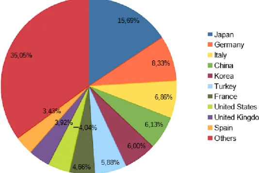
(6) Reference framework According to the Comtrade database of the United Nations (2016), the total amount of natural gas exports grew by 21% on average between 2009 and 2013. In last years, natural gas consumption has grown due to his abundance and to the fact that it is a cleaner fuel than oil, because it generates less CO 2 emissions. Furthermore, the improvement in storage facilities and transportation means have also contributed to this increase. Natural gas is a fossil fuel that is used, mostly, in the generation of electric and calorific power, and in plastic and fertilizer manufacturing (Schaffer, 2008). Thus, in 2013, according to the International Energy Agency (2015a), also known as IEA, natural gas represented 21.4% of global primary supply of energy, below coal (28.9%) and oil (31.1%). In that same year, natural gas accounted for 15.1% of global energy final consumption. In 2014, the leading producers of gas were the United States (with 20.7% of world total), Russia (18.3%), and Iran (4.8%). The main net exporters were Russia, Qatar and Norway, while the greatest net importers were Japan (mostly, due to the reduction in its production of nuclear energy after the Fukushima disaster), Germany and Italy, as it can be seen in figure 1. Figure 1. Main net importers of natural gas, 2014 (in percentage of world total).. Source: own elaboration with data from IEA (2015a). As a consequence of the high costs of transporting natural gas to long distances, it has not been possible to generate only one world price for this fuel, 6.

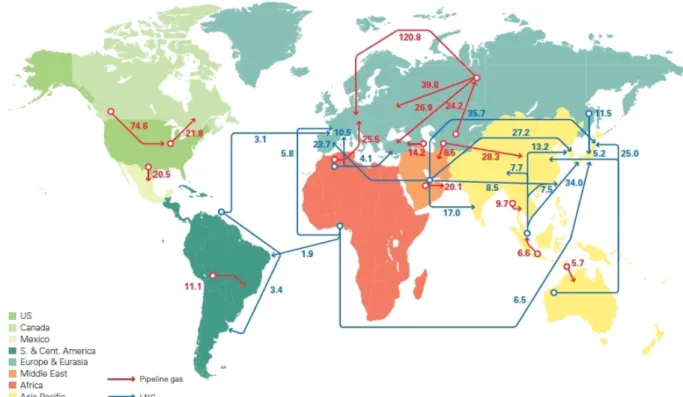
(7) although the markets are increasingly integrated and changes that happened in one of them are more rapidly reflected in others, according to what IEA states in its World Energy Outlook 2015. Traditionally, natural gas has been transported by pipelines, which has conditioned hugely its commerce. This fact made its market completely different to the market of another commodities which, because of their characteristics, are easier to transport. According to the classification that the IEA (2015b) does, we can divide the world in three main zones or markets for natural gas: North America, Asia – Pacific and Europe. Each zone has its own characteristics and systems to fix natural gas prices. In North America, the most important system for price fixing is the Henry Hub, which represents the movements of demand and supply inside the country. In Asia – Pacific, long-term contracts are the most common, and its prices are usually fixed to oil prices. In Europe, prices were fixed by long-term contracts too, and national markets worked, mostly, with a monopolistic system in which a single company was in charge of import, transport, storage and final distribution of natural gas. But, since the late 1990s, the European Commission is trying to change this kind of methods, turning to a system in which the competition between companies prevail and market barriers are eliminated. Most of the measures issued to improve competition are focused in reducing the highest market share that a single company can reach. This kind of price fixing system is already working in almost half of the European natural gas commerce (Chaton et al., 2012). In figure 2, it can be seen easily those areas of trade in natural gas, both compressed and liquefied. The first type, transported by pipelines, is carried out by countries located relatively close between them, while the liquefied natural gas (LNG) is usually transported to higher distances.. 7.

(8) Figure 2. World natural gas trade flows, 2014 (in billion cubic metres).. Source: Cedigaz, CISStat, FGE MENAgas service, GIIGNL, IHS Waterborne, PIRA Energy Group, Wood Mackenzie (n. d.); cited in BP (2015).. In this regard, the increase of liquefied natural gas trade represents a great innovation in the market of this fossil fuel because, due to its particular characteristics, makes its trade easier and opens a wide range of opportunities for the development of a global natural gas market. But, what is liquefied natural gas exactly? In accordance with Kumar et al. (2011), LNG is the cleaner type of natural gas, because it contains a 90% of methane, which allows that, when it is burned, it emits less quantity of CO2 than coal or oil. Following the explanation given by the authors, to produce LNG it is necessary to cool the natural gas to -161ºC, temperature at which it is liquefied and shrinked. This fact makes the natural gas easier to transport with LNG tankers, by sea, and with adapted containers, by road. Those LNG tankers and containers are loaded and unloaded in adapted facilities, that are located usually in ports. In these installations, when natural gas has to be sent, it is liquefied and loaded in ships or trucks (in this case, those facilities are known as liquefaction plants); but, when natural gas has to be received, it is unloaded, re-gasified and stored in the facilities themselves (called 8.

(9) regasification plants), being ready to be distributed to the consumption centres. This fact allows to transport LNG to a greater distance than compressed natural gas, and to build a real natural gas market around the world, because pipelines have several disadvantages that make them dangerous and useless for transporting natural gas to long distances (for example, their high economic cost requires the existence of a longterm contract between the producer region and the consumers to be cost-effective, they could be likely to generate political conflicts, they can not be built deeper than 100 metres under the sea…). For all these reasons, the authors expect that world demand for LNG grows faster than for total natural gas. In particular, the increase in consumption in Asia, mostly from China (the IEA1 highlights that, in 2035, Asian natural gas demand will be equal to the production of the United States nowadays), and its multiple applications, for example, in energy generation or as a fuel for vehicles with ecological engines, suggest to the authors that natural gas consumption in 2030 will be three times higher than it currently is. During 2014, the main exporters of LNG were Qatar, Malaysia, Australia, Nigeria and Indonesia, according to the data published in the BP Statistical Review of World Energy (2015). The main importers are also detailed in that report, and they were Japan, Republic of Korea, China, India and Taiwan. The prevalence of South-East Asia is obvious; the first country on this list that is not located in this area is Spain, in the sixth position. Natural gas demand is usually seasonal, but production is not, so producers increase their stock to moderate the quantity released to the market. Sometimes, that surplus of natural gas is liquefied to store it. Typically, the countries which export LNG have more natural gas than they need to consume, so, for them, to liquefy the gas is useful to store it and, later, sell it in international markets. The value chain of LNG is divided in four parts: production of natural gas (which accounts for 15-20% of total cost), liquefied (between 30-45% of the cost), loading and shipping (10-30% of the total cost) and storage and regasification (about 15-25% of total cost). The higher is the investment in the value chain, the higher is the innovation and the lower could be the total production cost, decreasing the price of the LNG (Maxwell and Zhu, 2011). 1 International Energy Agency, 2014. The Asian Quest for LNG in a Globalising Market.[pdf] International Energy Agency. Available at: https://www.iea.org/publications/freepublications/publication/PartnerCountrySeriesTheAsianQue stforLNGinaGlobalisingMarket.pdf [Accessed 10 February 2016] 9.

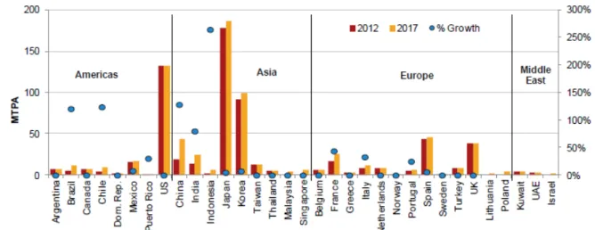
(10) As Wang and Notteboom (2010) detail, transportation costs of LNG depend directly of the distance between the liquefaction and the regasification plant. If LNG is transported in small containers, its flexibility to be traded increases, but it also increases its costs. The possibility of taking advantage from the economies of scale is higher in the process of storage. In fact, the biggest storage tanks that exist nowadays (480,000 cubic metres) are the ones that rise the optimum size. Furthermore, companies involved in the market are also increasing the size and capacity of the rest of the facilities in the LNG supply chain, with the objective of making profit from those economies of scale. In Figure 3 we can see the regasification capacity of the main participants in the LNG market in 2012 and their forecasts that they have to 2017. At this respect, Japan and the Republic of Korea, two big importers, are remarkable in the Asian zone, where we can also highlight the relative growth expected for Indonesia and China. In America, the United States has the biggest regasification capacity, and Chile and Brazil are expected to experience a great relative growth of their facilities to 2017. In the case of Europe, Spain and the United Kingdom have the highest regasification capacity in the region, which is not surprising, because the first is one of the main routes of entrance for natural gas to Europe, and the second has a strong industrial sector that consumes a large amount of this fuel. In the Middle East, as those countries are, mainly, natural gas exporters, they do not need regasification plants to receive LNG, but liquefaction plants to export it. Figure 3. Regasification capacity by country, 2012-2017 (in Million Tons Per Annum).. Source: PFC Energy Global LNG Service (n. d.), cited in International Gas Union, 2014.. 10.

(11) As it has been said previously, long-term contracts in natural gas markets have prevailed over another types. But, with the increase in LNG trade, which transport is more flexible and profitable over long distances, spot contracts have experienced a big expansion in recent years, after the liberalization of this market. However, it is expected that long-term contracts will still dominate the market, due to the fact that investors will want to secure the return of the large investment that is needed to build this kind of terminals, which are capital intensive (Wang and Notteboom, 2010). Thus, Cronshaw (2015) estimates that, by 2040, the five biggest producers of natural gas will jointly represent less than 50% of total natural gas quantity traded worldwide. By the same year, it is forecasted that LNG will represent about 50% of the total natural gas supply and demand. Another significant question that deserves to be analysed when a fossil fuel is studied, is the importance of energy security for the countries involved. To achieve the objective of energy security, countries need to increase the diversification of both their suppliers and energy sources. In this regard, LNG plays an important role, thanks to its flexibility to be traded, since it does not need an existing long-term agreement between the supplier and the consumer, so it makes easier its transport to large distances. In addition, as Wang and Notteboom (2010) point out, LNG also offers supply security, because it allows to change the provider easily if the latter suffers any problem. So, it can be said that LNG gives opportunities for the arbitrage in the international markets, allowing the buyers to look for the best price at any given time. A clear example of this concern about energy security is the one of the European Union, that imports most of the natural gas that it consumes by pipelines, mainly from Russia, Algeria and Norway. According to Locatelli (2015), the European Union should keep in mind this issue to avoid risks in its supply, because Russia and Algeria have internal political problems, and Ukraine, which is a transit country for natural gas, is immersed in a military conflict. In this situation, the European Union has opted to build new pipelines and regasification plants, with the objective of obtain new sources of supply. Schaffer (2008) states that Russia is not only a threat to the energy security of the European Union, but also for its independence in foreign policy, due to the fact that it is conditioned by the demands of Russia in order to maintain its natural gas supply. There are several countries involved in this geopolitical dispute, as the former soviet union republics, which are transit countries for natural gas, or Turkey. The latter has gained 11.

(12) relevance in this issue in the last years, due to the fact that the European Union has started the process to build a new pipeline, known as Nabucco Project, and another one through the Caspian Sea. Both new pipelines are expected to cross Turkey towards Europe. With those new infrastructures, the EU pretends to import natural gas from the Central Asian republics like Turkmenistan, from Azerbaijan or from Iran (Fatima, 2011). Under this scenario, LNG is presented as a good alternative to avoid the construction of those large infrastructures, which require an important expending and cross different countries, with the political inconveniences that it can generate. As it is usually transported from port to port, it avoids the fact that crossing several borders, with the costs that it imply in negotiations and trade agreements (Wang and Notteboom, 2010). Cohen (2007) highlights that LNG can be a good chance to diversify the energy sources of the European Union, thanks to the construction, particularly in Spain and Italy, of the regasification plants needed to transport and process this fuel.. 12.

(13) Literature review Literature about natural gas trade, and, specifically, about liquefied natural gas, is not very comprehensive, and many times it is focused on microeconomic aspects, like the article written by Harold, Lyons and Cullinan (2015), in which they study the determinants of residential demand for natural gas in Ireland. As the present research pretends to find out the characteristics related with international trade of natural gas, the literature review that has been done is focused in this field of study. Ackah’s research (2014), in which the determinants of natural gas demand in Ghana are analysed, highlights the importance of two main factors to study that demand. The first of these is the technological progress (like, for example, the improve in the efficiency of the equipment that consumes natural gas as fuel, or the improve in building insulation to prevent the heat from leaking). The second of this factors is the change in consumer preferences. The author applies two different models, one to estimate the residential demand and another one for the industrial demand, calculating for each one its own-price elasticity. Ackah concludes that changes in the income have a larger effect in natural gas consumption in the industrial sector rather than in the residential. In contrast, a greater change is produced in the residential demand when the price varies. In addition, the author shows that the industrial output and the final household spending affect significantly the natural gas demand. In this same way, Erdogdu’s research (2009) wants to estimate the determinants of natural gas demand in Turkey. This paper asserts that price elasticity of demand for natural gas is low, so the consumers do not respond strongly against changes in its price, and they do not substitute natural gas for another fuel when its price increases, either. Another paper that analyses the industrial natural gas consumption, in this case for Europe, is that of Andersen, Nilsen and Tveteras (2011). Here, the authors affirm that natural gas, traditionally, has been a good fuel to be consumed in stationary locations, like households or industrial plants, due to the need to be transported by pipelines. Furthermore, they point out the fact that some production plants, with the objective of being protected and adapted quickly to changes in prices, have installed systems that allow them to substitute the fuel that they use easily. These changes have been implemented, mainly, in energy-intensive industries, which are more affected by those changes in relative prices (the higher is the quantity of energy needed in the production process, the higher is the price elasticity that these sectors have). This 13.

(14) occurs mostly in British and Italian industries, which are powered mainly with natural gas. Andersen, Nilsen and Tveteras conclude that, in short-term, the demand of the companies studied is price inelastic, and it varies more between industries in the long term (authors affirm that there is heterogeneity between them and it has to be considered). Focused mainly in liquefied natural gas, the research done by Barnes and Bosworth (2015) applies the gravity equation to study the international trade of LNG around the world and its consequences in the natural gas global market. To develop the gravity model, they use a random effects estimation, so they can include variables that do not change over time, like the distance between two regions. The authors prove that LNG is now traded worldwide, while compressed natural gas is limited to regional markets isolated from each other. The results indicate that there is a huge evidence that, as the distance increases, the trade by pipeline is reduced, and the authors conclude that LNG has already decreased the regionalisation of the total natural gas market. In another article, Nick and Thoenes (2014) analyse the factors that affect natural gas prices. In it, the authors affirm that the study of this fuel is interesting for both private consumers (households) and industrial plants, due to the multiple uses that this commodity has. In their research, the empirical evidence shows that natural gas prices are affected by long-term variations in oil and coal prices, which act like substitute products. Another factor that the authors point out that affects natural gas prices is meteorology, but it has a transitory effect in the short term. Ritz (2014), details the reasons why, according to his research, there is not a real price arbitrage nowadays in natural gas markets. In the first place, he claims that many exporters do not allow their buyers to resell that gas to third parties, so the importers are not able to practice that kind of arbitrage. The author also explains the drawbacks about the capacity to transport LNG; despite the size of the tankers is increasing, their construction costs are very high, and most of them are linked to a concrete route by long-term contracts. Another factor that hinders arbitrage is, according to Ritz’s research, the fact that the LNG production and distribution chain is very complex, and it is not always owned by the same company. Thus, inconveniences of many types can emerge in diverse parts of the productive or transportation process, decreasing the flexibility and efficiency of the natural gas trade. Finally, the author points out another factors that can affect the arbitrage, like the time that can take for a 14.

(15) shipment to arrive to its final destination (and, thus, the possibility that during this period the prices vary significantly) or the quantities that can be transported (as LNG has to be transported in full tankers, it may be hard to find an available ship which transport capacity suits with the storage capacity that the importer has in a certain moment). Another type of articles can be found, focused in prediction models which can be applied to analyse the future of natural gas markets. In one of this papers, Egging et al. (2007) employ a model that embrace the entire supply chain of natural gas, both compressed and liquefied, using a sample of 52 countries, in which they try to predict the consequences that certain events could have in that market. Thus, if Russia cuts his exports to the European Union, the authors predict that global LNG trade will grow, and its price will rise too, due to the increase in imports that the EU would have to do. Furthermore, the authors assert that the competition between the United States and the European Union will be focused in the Atlantic zone, although the European countries will continue to depend on their imports by pipeline, setting aside the LNG only as an option to ensure their energy security. Following this line, Aune, Rosendahl and Sagen (2009), make some predictions about the world natural gas market until the year 2030, based on a model where they analyse several scenarios, taking into account different situations. The authors foresee an increase in global natural gas trade, due to the likely decrease in the European and North American reserves, which will lead them to increase their imports. The authors also predict a higher integration of prices in different international natural gas markets. These forecasts depend on the behaviour of the Middle East countries, because if them, which are big natural gas producers, act like a cartel, the prices in international markets will rise and this fuel trade will be affected. In the paper written by Egging, Holz and Gabriel (2009), they have developed a model in which predictions about natural gas markets can be made, taking into account the available facilities and the market characteristics. This model has been named as The World Gas Model. According to their calculations, Asia will be the continent with the higher trade in LNG, thanks to the increase that will be done in the needed infrastructures. Nevertheless, they also predict that the growth of LNG trade levels will experience a slowdown by 2020. The predictions made by Lochner and Bothe (2009), are focused mainly on three large consumer centres (Europe, the United States and Japan) that will have to 15.

(16) deal with large production and transportation costs. In this article, the authors forecast that, until 2030, compressed natural gas, which is traded by pipelines, will continue to be the main form to transport this fuel, although LNG could be cheaper in certain markets. Following the findings of the paper, Europe will continue to import its natural gas at a moderately low price, thanks to the construction of new pipelines that will connect the European continent with producer countries at a relative short distance. For its part, the United States, according to the predictions of the authors, will have to increase its supply diversification because of the depletion of its natural gas reserves. This fact will force the United States to import this fuel from several new countries: around 14 more suppliers, in accordance to the article. Japan depends heavily on natural gas imports, and the predictions show that it will continue to depend on them in the future. However, the Asian country will be benefited from the lower production cost of the facilities needed to trade with LNG and also from its geographic location, near some of the biggest natural gas producers in the world.. 16.

(17) The model In this paper, the determinants of natural gas world trade are going to be contrasted, with the aim to know what factors affect mainly the demand for this fuel. To achieve this as accurately as possible, two different gravity equations are going to be presented, one for the total natural gas, and another one only for the liquefied natural gas. Thus, for the selected period, global trade flows of this fuel are going to be analysed, according to the variables that best fit with each model. Gravity equations have been widely employed during the last years in many research papers related with trade, due to their simplicity and precision to determine the transportation costs. According to Reinert (2009), this model is based on an equation developed by Isaac Newton in his Gravity Law, in which he defined the gravitational force between two objects as a function of their respective masses and the distance between them, as it can be seen in equation (1):. GF ij =. Mi M j D ij. i≠j. (1). Where Mi and Mj are the masses of each object and Dij is the distance between them. Here, we can see that the gravitational force (GFij) between two bodies depends directly on their respective masses, but inversely on the existing distance between them. Following Reinert’s description, this type of equation has been applied on several research fields, like migrations or capital flows, but we are going to focus in the research done about international trade, which is our case. In accordance to the author, Tinbergen (1962) was the first paper that developed this kind of model, which was followed by Anderson (1979), Bergstrand (1985; 1989), Deardorff (1995) or Anderson and van Wincoop (2003). These papers gave a theoretical basis to the model, and they established the necessary conditions for its correct implementation. These models, related to international trade, replace the gravitational force for the trade volume between the country i and the country j, and the mass is represented with the income (sometimes, it can be substituted for the population 2 of each country or for the income per capita3). The distance remains, but now it represents how far are both countries between them, and it acts as a proxy of the transportation costs. Usually, with the 2. See Anderson (1979) or Reinert (2009).. 3. Bergstrand, J. H. 1985, “The Gravity Equation in International Trade: Some Microeconomic Foundations and Empirical Evidence”, The review of economics and statistics, vol. 67, no. 3, pp. 474-481. 17.

(18) objective of represent the elasticities between the dependent and independent variables with their coefficients, this equation is presented in its log linear form, so the function will look as follows:. ln Trade ij= β0 + β 1 ln Y i+ β2 ln Y j + β 3 ln Dist ij. i≠j. (2). Where Tradeij is the commercial flow between both countries, Yi is the income (usually, GDP) of the country i and Yj is the income of country j, while Dist ij is the distance between both regions. The expected values of β1 and β2 are positive, but for β3 is negative, being β0 a constant. As it has been said previously, two gravity equations are going to be presented in this paper, with the objective of studying the world natural gas trade and the determinants of its demand. In the first model, referring to total natural gas (whether or not liquefied), the trade flows between the ten main importers and ten main exporters of this fuel are going to be analysed, from 2010 to 2014, both included. To this end, the next equation has been developed:. lnTradeijt =β 0 + β 1 lnGDP it + β2 lnGDP jt + β 3 lnDist ij + β 4 lnOilprod jt + β 5 Indprcnt jt + + β 6 Comlangij + β 7 Eur j+ μ ijt i≠j. (3). t = 2010, 2011, 2012, 2013, 2014 In equation 3, Tradeijt represents the total exports from country i to j in t year,. which is the dependent variable that we are trying to explain. GDP it and GDPjt are the national income for each country in the year t, and the expected coefficient for both of them is positive, because we assume that the higher is the income, the higher is the trade. Distij is the distance between both regions, which obviously does not vary over time, and it is expected to affect negatively the commerce. Oilprod jt represents the oil production of the natural gas importer for each year. This variable is expected to reduce natural gas imports, because oil is a substitute fuel. Indprcnt jt represents the value added of the industry in percentage of the GDP for the importing country, and it is expected that a higher weight of the industry over the GDP increases natural gas imports. This variable is not represented in logarithms, because it is already calculated in percentage. Finally, two dummy variables are included in the model. The first one, Comlangij, takes value 1 if the importer and the exporter speak the same official language in both countries, and 0 if they do not. This variable is expected to have a positive coefficient, because if in both countries have the same language, the expected 18.

(19) transaction costs are lower. And the other dummy, Eur j, takes value 1 if the importing country is located in Europe and 0 otherwise, with the objective of studying if European countries import more natural gas than other regions. These two dummies are constant over the years. The second model pretends to study the trade flows in the liquefied natural gas market, and it is similar to the previous model: the trade between the ten main LNG importers and the ten main LNG exporters from 2010 to 2014, both included, will be studied. To carry out this research, the next equation has been created:. lnTradeijt =δ o +δ 1 lnGDP it +δ 2 lnGDP jt +δ 3 lnDist ij + δ 4 lnOilprod jt + δ 5 Indprcnt jt + +δ 6 Comlangij +δ 7 Reg jt +δ 8 Eur j + δ 9 Isl j+ ε ijt i≠j. (4). t = 2010, 2011, 2012, 2013, 2014 In equation (4), Tradeijt represents the LNG trade flow between the exporter i. and the importer j in year t, which is the dependent variable of the model. GDP it and GDPjt are the gross domestic product of each country in year t, and they are expected to affect positively the LNG imports, because the higher is the income, the higher should be the trade. Next variable is Dist ij, which represents the distance between each pair of countries (constant over time). It is expected to affect negatively the LNG trade. Oilprodjt represents the annual oil production of the LNG importer and it should reduce LNG imports. Indprcntjt is the value added by the industry of the importing country in percentage of the GDP for each year, and it is expected to have a positive coefficient. There are four dummy variables in this model. The first of them is Comlang ij, that takes value 1 if countries i and j have the same official language, and 0 if they do not. It is expected that countries with a common language trade more. The second dummy, Regjt, takes value 1 if the regasification capacity of the importing country is higher than the median of the sample, and 0 otherwise (for further details see the Data section). If a country has larger installed facilities, it should import more LNG, so this variable is expected to have a positive coefficient. As we have seen in papers like Cohen’s (2007), Europe considers LNG as a possibility to improve its energy security and supply diversification. For this reason, in this model a dummy variable called Eur j has been included, and it will take value 1 if the importing country is located in Europe and 0 if it is not. If Europe has a significant presence in LNG market, this variable should have a positive coefficient.. 19.

(20) Finally, Islj is a dummy that takes value 1 if the importing country is an island and 0 otherwise. Due to the difficulties to transport natural gas by pipelines across the sea (Kumar et al., 2011), it is expected that if a country does not have a land connexion with its suppliers, it would increase its imports of LNG. So, if this actually happens, this variable is expected to have a positive coefficient.. 20.

(21) Data In this section, we are going to explain all the details about the data used for the construction of the variables employed in each model, as the sources needed, the calculations made or the problems that have arisen during the process. In the first model, which analyses the total natural gas market between 2010 and 2014, the ten major importers and the ten major exporters of this fuel in 2014 were selected, with the data extracted from Comtrade, the United Nations database specialised in trade. From this data, the variable Tradeijt was built, and it represents the quantity of natural gas traded between each importer and exporter, in the year t. The quantities are expressed in kilograms. The ten main importers that have been selected are Japan, Germany, Republic of Korea, China, Italy, France, United States, Spain, United Kingdom and Belgium, while the ten major exporters are Qatar, Russia, Norway, Malaysia, Algeria, Netherlands, Indonesia, Australia, Canada and Nigeria. The data about the German imports were not disaggregated by countries, since the Comtrade database only provides the total quantity imported by Germany each year. To solve this problem, the Eurostat database was consulted. Here, the data were disaggregated by countries, but they were in million cubic metres. To adapt them to the variable built (in kilograms), the share imported from each country was calculated, and those proportions were applied to the total given by Comtrade. Thus, a good approximation of the German imports from each country in kilograms was made. Those trade flows are not constant over time, and some countries do not trade with others in any year of the study. Therefore, in this variable, which is the dependent in the model, we can find a great number of zeros, which could be problematic when making the estimation, as we will see later. The next variables that appear in the equation, GDP it and GDPjt, are the income of the exporting and the importing countries, and they were constructed with data from the database called World Development Indicators, of the World Bank. They are composed by the gross domestic product at market prices, in current US$, for each country in every year studied. Distij represents the distance between the capital cities of the exporter and the importer, in kilometres. These data were extracted from the CEPII database (Centre d’Études Prospectives et d’Informations Internationales, in French), which is a French institution that provides the necessary data for the research in international trade. The. 21.

(22) information needed to build the variable Comlangij, which indicates if the importer and the exporter share a common language, was also obtained from this database. Comlangij takes value 1 when both countries speak the same language, and 0 otherwise. Oilprodjt is a variable that measures the oil production of the importing country for each year (in thousands of barrels). The information needed for this variable was extracted from a database called JODI (Joint Organisations Data Initiative). The data were disaggregated by months and countries, and they were pooled to calculate the annual total for each country needed for the study. Indprcntjt represents the value added by the industry of the importing country in percentage of the gross domestic product, for each year. These figures were extracted from the World Development Indicators database, of the World Bank, but the quantities for the United States and Japan in 2014 did not appear. As this indicator has a very low variability from year to year (inter-annual variability for Japan between 2010 and 2013 was -0.9% on average, and it was 0.2% for the United States), we decided to introduce the average of the value added by the industry in percentage of the GDP from the previous four years as an approximate value for 2014. Initially, for calculating the effect in imports of the national industry, a variable that represented the total industrial production each year was included in the model, but it was removed because it generated perfect co-linearity due to, as the industrial production is part of the total GDP, it created a perfect linear relation with the national income. Finally, a dummy variable, Eurj, was included. This variable takes value 1 when the natural gas importer is located in Europe (in the sample selected, they are Germany, Italy, France, Spain, United Kingdom and Belgium), and value 0 otherwise. For the second model, which analyses the liquefied natural gas trade around the world, the same methodology has been followed. That means, the ten main importers and the ten main exporters of LNG in 2014 have been selected to analyse the trade between them from 2010 to 2014, both included. The selected ten greatest importers of this fuel are Japan, Republic of Korea, China, India, Taiwan, Spain, United Kingdom, Mexico, Brazil and Turkey. In the group of exporters we can find Australia, Indonesia, Malaysia, Nigeria, Qatar, Algeria, Oman, Russia, Trinidad and Tobago and Yemen. Both lists have been developed from the information published in the BP Statistical Review of World Energy 2015, where, among other details, the world LNG trade data are explained. 22.

(23) Once the country sample has been selected, the variable Tradeijt has been built, which represents the trade flows between country i and country j in year t, measured in kilograms. These figures have been extracted from the Comtrade database, which belongs to the United Nations. However, Taiwan, with a special legal status, does not appear in this database explicitly, but it does appear under the label “Other Asia, not elsewhere specified (NES)”, as the United Nations themselves explain 4, so these data have been used in the research. In addition, the proportions of the imported quantity from each country given by this database are in line with the proportions in billion cubic metres that can be calculated for Taiwan from the information in the BP Statistical Review of World Energy 2015. Moreover, the data from Turkey does not appear in this database. This case is different from the previously commented of Germany, because now we do not have any data, not even the annual total. Thus, the data about the Turkish imports of liquefied natural gas were extracted from Eurostat. As those data were in billion cubic metres, we had to convert them to kilograms, like the rest of data in this variable. In order to do this, we use the conversion factor published by the Ministry of Finances from the British Columbia (Canada), which states that 1 kilogram of natural gas is equal to 1,406 cubic metres. In this case, the variables that coincide with the first model (GDP it, GDPjt, Distij, Oilprodjt, Indprcntjt, Comlangij and Eurj) have been obtained from the same sources, and they also have been built similarly as for the first model. However, with the GDP and the value added by the industry in percentage of the GDP, we had the same problem with Taiwan as before with its LNG imports; those data from the Asian country did not appear in the World Development Indicators database of the World Bank. The GDP of Taiwan from 2010 to 2014 has been extracted from Index Mundi database, which uses information from the CIA World Factbook. For the value added by the Taiwanese industry in percentage of its GDP, we have consulted the Index Mundi database again, but also the CIA World Factbook itself. Furthermore, for both Taiwan and Japan (as it happened in the previous model), the value of this variable for 2014 has been calculated with the average of the previous four years, thanks to the low inter-annual variability of this indicator.. 4. See: http://unstats.un.org/unsd/tradekb/Knowledgebase/Taiwan-Province-of-China-Tradedata 23.

(24) A similar problem has arisen with Yemen, which GDP for 2014 did not appear in the data provided by the World Bank. Here, the growth rate of its GDP in 2014 has been extracted from the CIA World Factbook, which was -0.2%. Thus, having the GDP value in 2013, the growth rate has been applied to obtain a good approximation for the GDP of Yemen in 2014. To create the dummy variable Reg jt, the data about the regasification plants in each country and their storage capacity, measured in million tonnes per annum, were extracted from the World LNG Report, published by the International Gas Union (IGU) in 2016. To collect the effect that these facilities have in the LNG trade, the median storage capacity of the selected importing countries for each year has been calculated. Then, value 1 has been given for the countries which have a storage capacity higher than the median, and value 0 has been given for the countries with a storage capacity under the median. The median has been chosen instead of the mean due to the great difference between the high storage capacity of Japan and Korea over the rest of the sample, with a lower capacity. This fact provoked that only two or three countries were over the mean, so the variable may not be significant (for further information, see Annexes 1 and 2). For the variable Eurj, value 1 has been given to the importing countries located in Europe, which in this sample are Spain, United Kingdom and Turkey (the latter has been included due to its geographic proximity and because it is a transit zone for the natural gas addressed to Europe5), and value 0 has been given for the rest of the world importers. Similarly, the variable Isl j has been built, giving value 1 for countries located in islands (in this case, Japan, Taiwan and the United Kingdom) and value 0 for the countries located in a continent. Obviously, those last two dummies are constant over time.. 5. As it has been cited previously, the papers of Fatima (2011) or Schaffer (2008), for example, make a comprehensive analysis of this issue. 24.

(25) Econometrics In this section, we are going to explain everything related to the econometrics used in the estimations, like the organisation of the data, the statistical software or the type of models applied. As it has been mentioned above, the data is organized as a panel, with ten importers and ten exporters, which brings a total of a hundred observations each year, from 2010 to 2014. So, there is a total of five hundred observations in the panel. But, as we have explained in the Data section, many of those pairs of countries did not trade natural gas during the period selected, so we will have an unbalanced panel. The software used is Gretl, a statistical open-source package. For each model, we are going to apply two estimation methods: Pooled Ordinary Least Squares (OLS) and Random Effects (RE). This method is the same as Barnes and Bosworth (2014) followed in their research, where they also employed a gravity equation. The first of them, pooled OLS, is one of the most common econometric techniques, due to its simplicity and clarity in offering the results. The second, RE, is used for panel data regressions, and it allows to include time-constant variables, in contrast with the Fixed Effects estimator, where this kind of variables are excluded. This fact is very important for this research, because important time-constant variables have to be contrasted.. 25.

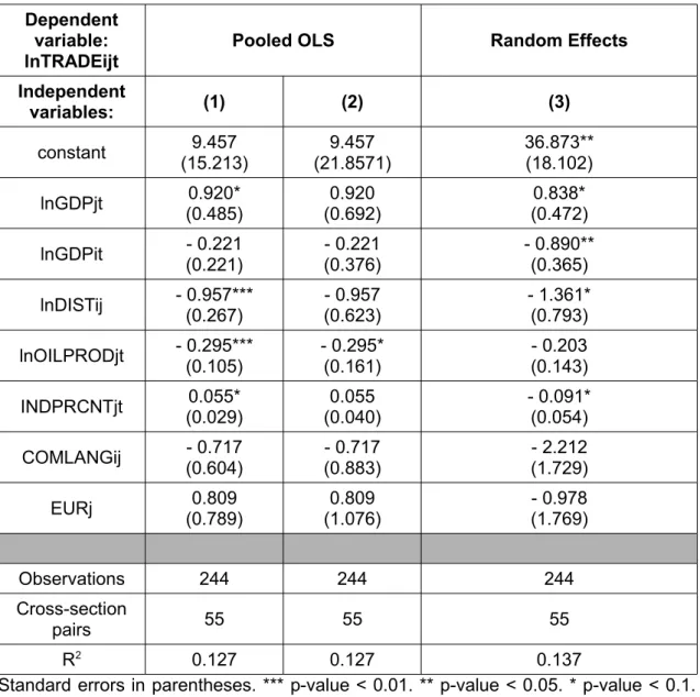
(26) Results The results of the regressions are going to be presented in the next pages, for both models. In the first place, we are going to analyse the results for the model that covers the total natural gas market. Figure 4. Results of the regressions made with the total natural gas market model. Dependent variable: lnTRADEijt. Pooled OLS. Random Effects. Independent variables:. (1). (2). (3). constant. 9.457 (15.213). 9.457 (21.8571). 36.873** (18.102). lnGDPjt. 0.920* (0.485). 0.920 (0.692). 0.838* (0.472). lnGDPit. - 0.221 (0.221). - 0.221 (0.376). - 0.890** (0.365). lnDISTij. - 0.957*** (0.267). - 0.957 (0.623). - 1.361* (0.793). lnOILPRODjt. - 0.295*** (0.105). - 0.295* (0.161). - 0.203 (0.143). INDPRCNTjt. 0.055* (0.029). 0.055 (0.040). - 0.091* (0.054). COMLANGij. - 0.717 (0.604). - 0.717 (0.883). - 2.212 (1.729). EURj. 0.809 (0.789). 0.809 (1.076). - 0.978 (1.769). Observations. 244. 244. 244. Cross-section pairs. 55. 55. 55. R2 0.127 0.127 0.137 Standard errors in parentheses. *** p-value < 0.01. ** p-value < 0.05. * p-value < 0.1. Source: own elaboration.. As it has been said previously, the great number of zeros that the dependent variable contains provokes that we have an unbalanced panel of 244 observations. In the first model, we can see that the coefficient of the GDP of the importer is positive and significant at a 10% level. It means that the higher is the national income in the importing country, the higher are their natural gas imports. The distance between the. 26.

(27) importer and the exporter and the oil production of the importer have both a negative coefficient, significant at a 1% level. Thus, the longer is the distance, the lower is the trade between countries; and, the higher is the production of oil in the importing country, the lower are their natural gas imports. We also have a positive and significant at a 10% level coefficient for the value added by the industry, which means that as a country increases its industry, it also increases its natural gas imports. But we have some problems in this model. For example, the R-squared is very low, and this means that the independent variables selected only explain the 12.69% of the dependent variable movements. And, furthermore, if we apply the White contrast to see if there is presence of heteroscedasticity, we obtain a p-value of 0.000937, rejecting the null hypothesis of homoscedasticity. Then, the coefficients obtained are unbiased, but they are inefficient, so the t-statistics are invalid (Wooldridge, 2006). To solve this problem, we apply a regression that is robust to heteroscedasticity, as we can see in model (2). Here, the coefficients are the same as in model (1), but the significance levels have changed, because, as it has been said, the t-statistics are now different. Now, in the second model, we can see that there is only one significant variable, the oil production of the importer, at a 10% level. The sign is negative, as it has been expected, which means that if a country increases its oil production, it will reduce its natural gas imports. When the random effects estimator is applied, we can see that the GDP of the importing country has a positive coefficient, and it is significant at a 10% level. This means that, in this case, if the GDP of the importer increases by 1%, it is predicted that its natural gas imports will rise by 0.84%, according to the results. The coefficient of the GDP of the exporter is negative and significant at a 5% level. So, in our case, the sign of this coefficient is unexpected, and it would be due to our little sample of exporting countries or because countries with low GDP export more commodities, like natural gas. The distance plays a negative role in natural gas trade, and its coefficient is negative and significant at a 10% level. In particular, an increase by 1% in the distance between two countries is predicted to decrease the trade of those countries by 1.36%. The coefficient of the variable that measures the value added by the industry is negative and significant at a 10% level. This is not the expected sign and it would require further research, but we think that it could be caused by our limited sample. When we look at the Breusch-Pagan contrast, we can see that the null hypothesis is rejected at every significance levels, so we conclude that random effects is preferred to pooled OLS. This is because we can assume that the variance of the error term has an unobservable component (Wooldridge, 2006). Then, when we 27.

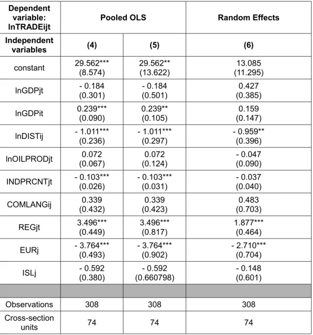
(28) analyse the Hausman test we can observe that at a 1% level of significance, the null hypothesis is not rejected, so random effects is preferred to fixed effects because the estimators are not biased and random effects estimator is more efficient. But, at a 5% and 10% level of significance, the null hypothesis is rejected, and then, fixed effects is better than random effects, due to the fact that the estimators of both models are significantly different and fixed effects is better than random effects. In our case, as we want to include some important time-constant variables, the random effects estimator has been chosen (Barnes and Bosworth, 2015). Now, we are going to analyse the models referring to the LNG trade. Figure 5. Results of the models applied to study the LNG market. Dependent variable: lnTRADEijt. Pooled OLS. Random Effects. Independent variables. (4). (5). (6). constant. 29.562*** (8.574). 29.562** (13.622). 13.085 (11.295). lnGDPjt. - 0.184 (0.301). - 0.184 (0.501). 0.427 (0.385). lnGDPit. 0.239*** (0.090). 0.239** (0.105). 0.159 (0.147). lnDISTij. - 1.011*** (0.236). - 1.011*** (0.297). - 0.959** (0.396). lnOILPRODjt. 0.072 (0.067). 0.072 (0.124). - 0.047 (0.090). INDPRCNTjt. - 0.103*** (0.026). - 0.103*** (0.031). - 0.037 (0.040). COMLANGij. 0.339 (0.432). 0.339 (0.423). 0.483 (0.703). REGjt. 3.496*** (0.449). 3.496*** (0.817). 1.877*** (0.464). EURj. - 3.764*** (0.493). - 3.764*** (0.902). - 2.710*** (0.704). ISLj. - 0.592 (0.380). - 0.592 (0.660798). - 0.148 (0.601). Observations. 308. 308. 308. Cross-section units. 74. 74. 74. 28.

(29) Dependent variable: lnTRADEijt Independent variables. Pooled OLS (4). Random Effects (5). (6). R2 0.410 0.410 0.347 Standard errors in parentheses. *** p-value < 0.01. ** p-value < 0.05. * p-value < 0.1. Source: own elaboration.. For these regressions, we have an unbalanced panel with 308 observations, due to the fact that the dependent variable Tradeijt has many 0 values. In the model number 4, with pooled OLS, we have that the coefficients of the GDP of the exporter, the distance between both countries, the value added by the industry of the importer, the regasification plants dummy and the Europe dummy are significant at a 10%, 5% and 1% level. The sign for the GDP of the exporter is positive, as expected in the Model section above, but in contrast with the result obtained in the total natural gas model. This change may be due to the high construction cost of the liquefaction plants needed to export LNG, which poorer countries probably can not afford. We can also see that the distance affects negatively the liquefied natural gas trade, according to our forecasts (following our results, if the distance increases by 1%, the LNG trade between two countries will decrease by 1.01%). The sign for the value added by the industry of the importer in percentage of the GDP is surprisingly negative, as we expected it to be positive. Further research should be done in this sense. The regasification plants dummy that has been included has the expected effect, and suggests us that countries with a regasification capacity over the median import more LNG, remarking the importance of the adapted facilities in this kind of commerce. On the contrary, we can see that the dummy that indicates if the importer is European has a negative coefficient, which means that Europe has still a low weight in the international trade of LNG. The R-squared of the regression indicates that around 41% of the variation of Tradeijt is explained by the variables included in the model. But, as before in the total natural gas model, we have a problem with the heteroscedasticity. When the White contrast is applied, the null hypothesis of homoscedasticity is rejected, so we should apply a model with robust estimators, as in the model (5). When estimating this robust estimators, as we have already explained, the coefficients and R-squared do not change, but the standard deviation and the tstatistics do. So, the level of significance changes in our model for the constant and for the GDP of the importer, both being significant at a 5% and 10% level. As everything 29.

(30) else remains as before, the interpretation of the parameters of the model is the same as for model (4) given previously. As there are only little changes when robust estimators regression is applied, we can think that heteroscedasticity is less problematic in model (4) than in model (1). Now, going to the random effects estimator, we can see that only three variables are significant. The first of them, the distance, has the expected sign, negative, as we have already explained, and it is significant at a 10% and 5% level. For a 1% increase in distance between two countries, the model forecasts a reduction of around 0.96% in their LNG trade. Again, the regasification plants dummy is significant at every levels, but its coefficient is now lower than before with pooled OLS. The dummy for the European countries has a negative sign, as in model (5), which confirms our theory about the low weight of Europe in this market. As it has been done before, the Breusch-Pagan test has been analysed. Again, the random effects estimator is preferred over the pooled OLS method, and it is also chosen instead fixed effects for the same reason as before; we need to include some important time-constant variables in our models, which would be eliminated with the fixed effects estimator.. 30.

(31) Conclusions In this study, the determinants of the demand for natural gas and LNG have been analysed, using two different models based on the gravity equations. In the first place, a Reference Framework has been presented, with the objective of providing a technical and descriptive basis for the reader who is not specialised in energy economics or in the natural gas market. The theoretical basis and different researches in the natural gas and LNG field is given in the Literature Review section. The following section has explained the models used, with a brief literature review about the gravity equations and the description of the variables included in both models. In the Data section, everything related to the construction of the variables used, the data sources and the problems found during this process has been explained and detailed. The next point has explained the econometric methods applied in the regressions, the data organisation and the statistical package used. And finally, the findings of the regressions have been stated in the Results section. The most relevant conclusion that can be reached from this paper is that the distance between two countries conditions greatly their natural gas trade. In five of the six models analysed, the coefficient for this variable has been negative and statistically significant, which means that the empirical evidence suggests that the further away an importer is from an exporter, the lower is the natural gas trade between them. Another important finding of this paper is the fact that, in the liquefied natural gas market, the adapted facilities play a key role in the trade of this fuel. We can observe a strong empirical evidence that, if a country has a regasification capacity over the median value, it will import more LNG. It would be interesting to make a deeper study about the impact of infrastructures in the LNG trade in future research. We can also see that the European market of LNG is not relevant yet. This dummy variable in the LNG model has a negative and significant sign, which means that European countries import less LNG than the other countries in the sample. This result, combined with the fact that Europe is the region with the greatest natural gas imports by pipeline (BP, 2015), makes us believe that the relative weight of LNG in the total natural gas market is still low for the European continent. It may be interesting to follow the evolution of this market in the future. However, some results differ from the predictions made in the Model section. Surprisingly, the variable that represents the value added by the industry of the. 31.

(32) importer in percentage of the GDP in the LNG model is negative and significant in the Pooled OLS regression and in the Random Effects regression in the total natural gas model. It may be due to the limited sample used, but further investigation should be done about it. Another result that was not expected is the negative sign of the coefficient for the GDP of the importer with the Random Effects estimation in the total natural gas model. The fact that poor countries usually export more commodities than rich countries may explain this. But, in the model that is focused in the LNG market, the regression of Pooled OLS gives us a positive and significant coefficient for this same variable. It may be explained because the infrastructures needed to liquefy natural gas to sell it are very expensive, and poor countries can not afford those great costs. Finally, we have already seen the problem with the presence of many zeros in the dependent variables. It is caused by the special characteristics of this fuel, which needs adapted infrastructures to be transported and stored. These features also cause that the natural gas market is ruled by long-term contracts, so some countries import the natural gas that they need from the same countries during the period selected, and never import it from others. This is slowly changing thanks to the LNG, which allows to import natural gas with spot contracts, making its market more flexible and diversified (the number of observations in the LNG model, 308, indicates that its dependent variable contains less zero values than the dependent variable of the total natural gas model, which has only 244 observations).. 32.

(33) References Ackah, I., 2014. "Determinants of natural gas demand in Ghana", OPEC Energy Review, vol. 38, no. 3, pp. 272-295. Andersen, T.B., Nilsen, O.B. & Tveteras, R., 2011. "How is demand for natural gas determined across European industrial sectors?", Energy Policy, vol. 39, no. 9, pp. 5499. Anderson, J.E., 1979. “A Theoretical Foundation for the Gravity Equation”, American Economic Review, vol. 69, no. 1, pp. 106-116. Anderson, J.E. & van Wincoop, E., 2003. "Gravity with gravitas: A solution to the border puzzle", The American Economic Review, vol. 93, no. 1, pp. 170-192. Aune, F., Rosendahl, K., & Sagen, E., 2009. “Globalisation of Natural Gas Markets – Effects on Prices and Trade Patterns”, The Energy Journal, vol. 30, pp. 39. Barnes, R. & Bosworth, R., 2015. "LNG is linking regional natural gas markets: Evidence from the gravity model", Energy Economics, vol. 47, pp. 11. Bergstrand, J.H., 1985. “The Gravity Equation in International Trade: Some Microeconomic Foundations and Empirical Evidence”, The Review of Economics and Statistics, vol. 67, no. 3, pp. 474-481. Bergstrand, J.H., 1989. “The Generalized Gravity Equation, Monopolistic Competition, and the Factor-Proportions Theory in International Trade”, The Review of Economics and Statistics, vol. 71, no. 1, pp. 143-153. BP, 2015. BP Statistical Review of World Energy. [pdf] BP. Available at: http://www.bp.com/content/dam/bp/pdf/energy-economics/statistical-review-2015/bpstatistical-review-of-world-energy-2015-natural-gas-section.pdf. [Accessed. 30. April. 2016] Centre d’Études Prospectives et d’Informations Internationales, 2016. Gravity Database.. [online]. Available. http://www.cepii.fr/CEPII/en/bdd_modele/presentation.asp?id=8. at: [Accessed. 8. May. 2016] Chaton, C., Gasmi, F., Guillerminet, M. & Oviedo, J., 2012. "Gas Release and Transport Capacity Investment as Instruments to Foster Competition in Gas Markets", Energy Economics, vol. 34, no. 5, pp. 1251-1258. 33.

(34) Central Intelligence Agency, 2016. The World Factbook. [online] Available at: https://www.cia.gov/library/publications/the-world-factbook/ [Accessed 21 May 2016] Cohen, M.D., 2007. "Russia and the European Union: An Outlook for Collaboration and Competition in European Natural Gas Markets", Demokratizatsiya, vol. 15, no. 4, pp. 379-390. Cronshaw, I., 2015. "World Energy Outlook 2014 projections to 2040: natural gas and coal trade, and the role of China", Australian Journal of Agricultural and Resource Economics, vol. 59, no. 4, pp. 571-585. Deardorff, A.V., 1995. Determinants of Bilateral Trade: Does Gravity Work in a Neoclassical World?, National Bureau of Economic Research, Inc, NBER Working Papers: 5377. Egging, R., Gabriel, S.A., Holz, F. & Zhuang, J., 2007. A Complementarity Model for the European Natural Gas Market, Federal Reserve Bank of St Louis, St. Louis. Egging, R., Holz, F. & Gabriel, S.A., 2009. The World Gas Model: A Multi-Period Mixed Complementarity Model for the Global Natural Gas Market, Federal Reserve Bank of St Louis, St. Louis. Erdogdu, E., 2009. Natural gas demand in Turkey, Federal Reserve Bank of St Louis, St. Louis. European Commission, 2016. Eurostat Database. [online] Available at: http://ec.europa.eu/eurostat [Accessed 5 May 2016] Fatima, M., 2011. "Trends in Economic and Trade Relations between Russia and the European Union", Journal of European Studies, vol. 26-27, no. 2-1. Harold, J., Lyons, S. & Cullinan, J., 2015. "The determinants of residential gas demand in Ireland", Energy Economics, vol. 51, pp. 475. Index. Mundi,. 2016.. IndexMundi.. [online]. Available. at:. http://www.indexmundi.com/ [Accessed 21 May 2016] International Energy Agency, 2014. The Asian Quest for LNG in a Globalising Market.. [pdf]. International. Energy. Agency.. Available. at:. https://www.iea.org/publications/freepublications/publication/PartnerCountrySeriesTheA sianQuestforLNGinaGlobalisingMarket.pdf [Accessed 10 February 2016] 34.

(35) International Energy Agency, 2015a. Key World Energy Statistics. [pdf] International. Energy. Agency.. Available. at:. https://www.iea.org/publications/freepublications/publication/KeyWorld_Statistics_2015. pdf [Accessed 29 March 2016] International Energy Agency, 2015b. World Energy Outlook 2015. [pdf] International. Energy. Agency.. Available. at:. http://www.worldenergyoutlook.org/weo2015/#d.en.148701 [Accessed 29 March 2016] International Gas Union, 2014. Natural gas facts & figures. [pdf] International Gas. Union.. Available. at:. http://www.igu.org/sites/default/files/Part%203(Oct14)-. %20LNG.pdf [Accessed 10 February 2016] International Gas Union, 2016. 2016 World LNG Report. [pdf] International Gas Union. Available at: www.igu.org/download/file/fid/2123 [Accessed 17 May 2016] Joint Organisations Data Initiative, 2016. JODI Oil World Database. [online] Available. at:. http://www.jodidb.org/ReportFolders/reportFolders.aspx?. sCS_referer=&sCS_ChosenLang=en [Accessed 14 May 2016] Kumar, S., Kwon, H., Choi, K., Cho, J.H., Lim, W. & Moon, I., 2011. "Current status and future projections of LNG demand and supplies: A global prospective", Energy Policy, vol. 39, no. 7, pp. 4097. Locatelli, C., 2015. "EU-Russia trading relations: the challenges of a new gas architecture", European Journal of Law and Economics, vol. 39, no. 2, pp. 313-329. Lochner, S. & Bothe, D., 2009. "The development of natural gas supply costs to Europe, the United States and Japan in a globalizing gas market – Model-based analysis until 2030", Energy Policy, vol. 37, pp. 1518-1528. Maxwell, D. & Zhu, Z., 2011. "Natural gas prices, LNG transport costs, and the dynamics of LNG imports", Energy Economics, vol. 33, no. 2, pp. 217. Ministry of Finance of British Columbia, 2013. Conversion factors for fuel. [pdf] Ministry. of. Finance. of. British. Columbia.. Available. at:. http://www.sbr.gov.bc.ca/documents_library/shared_documents/Conversion_factors.pdf [Accessed 5 May 2016] Nick, S. & Thoenes, S., 2014. "What drives natural gas prices? - A structural VAR approach", Energy Economics, vol. 45, pp. 517.. 35.

(36) Reinert, K.A., 2009. Gravity models, Princeton University Press, Princeton. Ritz, R.A., 2014. "Price Discrimination and Limits to Arbitrage: An Analysis of Global LNG Markets", Energy Economics, vol. 45, pp. 324-332. Schaffer, M.B., 2008. "The great gas pipeline game: monopolistic expansion of Russia's Gazprom into European markets", Foresight: the Journal of Futures Studies, Strategic Thinking and Policy, vol. 10, no. 5, pp. 11-23. Tinbergen, J., 1962. Shaping the World Economy: Suggestions for an International Economic Policy. New York: Twentieth Century Fund. United. Nations,. 2016.. Comtrade. Database.. [online]. Available. at:. http://libweb.anglia.ac.uk/referencing/harvard.htm [Accessed 5 May 2016] Wang, S. & Notteboom, T., 2010. World LNG shipping: dynamics in markets, ships and terminal projects. In: Current Issues in Shipping, Ports and Logistics. Brussels: University Press Antwerp. Ch. 7. Wooldridge, J.M., 2006. Introductory econometrics: A modern approach. 4th ed. Mason: South-Western Cengage Learning. World Bank, 2016. World Development Indicators Database. [online] Available at: http://data.worldbank.org/data-catalog/world-development-indicators [Accessed 14 May 2016]. 36.

(37) Annexes Annex 1. Data used for the Regjt dummy (in million tonnes per annum). CAPACITY (MT Japan Korea China India Taiwan Spain UK Mexico Brazil Turkey. 2010 179 91,3 14,7 15 13 43,9 38 12,9 1,9 10,3. 2011 179 91,3 21,2 15 13 43,9 38 12,9 1,9 10,3. 2012 182,7 91,3 22,2 15 13 43,9 38 16,7 7,9 10,3. 2013 184,7 91,3 34,4 22 13 49,3 38 16,7 7,9 10,3. 2014 188,2 98,1 39,4 22 13 49,3 38 16,7 11,7 10,3. Mean Median. 42 14,85. 42,65 18,1. 44,1 19,45. 46,76 28,2. 48,67 30. Source: own elaboration with IGU (2016) data.. Annex 2. Values of the Regjt dummy. Dummy median Japan Korea China India Taiwan Spain UK Mexico Brazil Turkey. 2010 1 1 0 1 0 1 1 0 0 0. 2011 1 1 1 0 0 1 1 0 0 0. Source: own elaboration.. 37. 2012 1 1 1 0 0 1 1 0 0 0. 2013 1 1 1 0 0 1 1 0 0 0. 2014 1 1 1 0 0 1 1 0 0 0.

(38)