Wind turbine multivariable optimal control based on incremental state model

WIND TURBINE MULTIVARIABLE OPTIMAL CONTROL BASED ON

INCREMENTAL STATE MODEL

Jose Miguel Adanez Basil Mohammed Al-Hadithi Agustin Jimenez

ABSTRACT

The multivariable optimal control of a wind turbine by an approach based on incremental state model is proposed. The advantages of incremental state model in comparison with the non incremental one are that the control action cancels steady state errors and incremental state solves the problem of computing the target state, choosing zero as an objective. Linear Quadratic Regulator (LQR) and optimal state observer are applied. The effectiveness of the proposed control method, over the non incremental one, is examined by applying the linear controllers to the nonlinear wind turbine model. The results show that incremental LQR control presents good transient response and zero steady state errors, even in presence of disturbances, nonlinearities and modelling errors.

I. INTRODUCTION

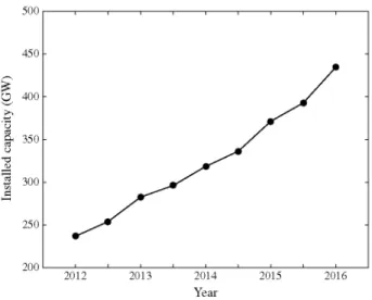
Wind turbine technology has undergone rapid development in response to increased demand for renew-able energy. At the beginning of 2017, installed capacity worldwide was about 485 GW, see Fig. 1, installing more than 50 GW in 2016 [1]. Technological advances in wind turbines make necessary the design of effective control systems, whose main objective is to get the maximum pos-sible energy and to increase the wind turbine lifetime by minimizing loads at the structure [2].

There are several control loops responsible of opti-mum operation of the wind turbine [3,4]: rotor angular speed control; torque control [5]; pitch control (angle of blades) [6]; yaw control (orientation of the wind tur-bine) [7]; and power control loops [8]. Currently, the problem of wind turbine control in industry is solved by implementing each control loop separately using conven-tional proporconven-tional integral (PI) or proporconven-tional integral derivative (PID) controllers [9], and minimizing the cou-plings among loops by iterative adjustments. However,

the new wind turbine structures, larger, more flexible and operating in uncertain environments, make traditional controllers designs insufficient. Therefore the need for advanced control methods are increased [10,11].

Although the wind turbine industry mainly uses classical controllers, some researchers have also tried some modern control techniques. For example, a Quan-titative Feedback Theory (QFT) controller has been applied in an industrial turbine [12]. Also, multivari-able state space H ^ control has been tested in the tur-bine CART 3 (Controls Advanced Research Turtur-bine 3-bladed) with very promising results [13,14].

The speed control of induction motor fed by wind turbine using imperialist competitive algorithm is pro-posed in [15]. The propro-posed design problem of speed controller is established as an optimization problem. Imperialist competitive algorithm is adopted to search for optimal controller parameters by minimizing the time domain objective function.

In [16], the authors propose Ant Lion optimization algorithm for optimal allocation and sizing of renewable distributed generation sources in various distribution networks. Allocation and sizing of distributed genera-tion have greatly affected on the system losses. Photo-voltaic systems and wind turbines are considered here as sources of distributed generation. The most appropri-ate candidappropri-ate buses for installing distributed generation are suggested using loss sensitivity factors and the algo-rithm is employed to deduce the locations of distributed generation and their sizing from the elected buses.

500 i , , , , , , , , , 1

450

-* /

O, 400 - V

% 350 - /

3 300 - m'

HH Jt

250 - ^ ^ *

2 0 0 I 1 1 1 1 1 1 1 1 1 2012 2013 2014 2015 2016

Year

Fig. 1. Total installed capacity.

nonlinear controller is designed to meet two main con-trol objectives, the speed reference optimization in order to extract a maximum wind energy whatever the wind speed, and power factor correction to avoid net har-monic pollution. These objectives are achieved despite the mechanical parameters uncertainty.

A cascaded multivariable nonlinear control is per-formed in [18]. The inner loop controls the generator torque and stator flux, while the outer loop controls the rotor angular speed.

In [19], a classical multivariable control is devel-oped by decoupling and feedforward compensation. The decoupling is incorporated to minimize interaction effects among classical PI control loops. Feedforward compensator is included to reduce the effects of wind disturbances and electrical load changes.

Multivariable coupling effects are studied for load reduction in wind turbines [20]. They prove that multiple single-input single-output (MSISO) controller is easy to understand but it creates couplings among control loops, and it has to be improved by iterative adjustment. On the other hand, multi-input multi-output (MIMO) controller in state space form can achieve higher load reductions without any additional filtering.

A gain scheduling method based on output interpo-lation of some local controllers independently designed is presented for wind turbine control [21]. The local con-trollers are designed using H ^ optimal control method for the multivariable state space model defined at each local point.

An optimal control system based on feedforward and state-feedback controller is designed for a fuel processing system [22], using a loop transfer recovery method and a generalized linear quadratic Gaussian

method. A new methodology is proposed to design dig-ital PID controllers for multivariable systems with time delays [23]. Most of the parameters are systematically tuned using state-feedback and state-feedforward LQR approach. An extension for multiple time delays is pre-sented in [24].

In [25], the authors investigates the problem of finite-time optimal tracking control for dynamic systems on Lie groups for the situation when the tracking time and the cost functions need to be considered. A control law is designed to track a desired reference trajectory at the given time and to guarantee the cost functions to be optimal.

A design strategy of robust disturbance observer is proposed systematically for stable non-minimum phase systems in [26]. This strategy synthesizes the internal and robust stability, relative order and mixed sensitiv-ity design requirements together to establish the opti-mization function. The optimal solution is obtained by standard H ^ control theory under the condition of guar-antying the presented requirements.

In [27], a predictive control algorithm called Differ-ence Equation Matrix Model (DEMM) was developed and applied to the control of a wind turbine. This algo-rithm is considered a mixture of Dynamic Matrix Con-trol (DMC) [28] and Recursive Generalized Predictive Control (RGPC) [29]. Several advantages over the two methods are obtained. In comparison with [28], DEMM control decreases the computational cost, which make it compatible for real time applications. Also, comparing with [29], DEMM control presents zero steady state error, good and robust performance in front of disturbances and model uncertainties.

The incremental state model is presented in [30] to model multivariable nonlinear delayed systems expressed by a generalized version of the Takagi-Sugeno (T-S) fuzzy model. The advantages of the incremental state model compared with the non-incremental one have been defined. First, it solves the problem of computing the target state, choosing zero incremental state as an objec-tive. Second, the control action in an incremental form is equivalent to introduce an integral action. Third, incre-mental state model makes the affme terms disappear.

In [30] a new optimal state observer is also pre-sented. In this way, and combined with the LQR method [31,32], a local optimization is produced at each operat-ing point defined by the T-S fuzzy model. A multivariable thermal mixing tank system is chosen to evaluate the effectiveness of the proposed methods.

Results of proposed control algorithms applied to the wind turbine model are shown and analyzed in Section IV. Finally, the conclusions are presented in Section V. The nomenclature is added in the appendix in Table Al and the list of abbreviations is added in Table A2.

II. WIND TURBINE M O D E L

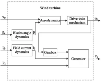
In this section, the wind turbine dynamic model is described. The block diagram, see Fig.2, represents the multivariable behaviour of the wind turbine. The sys-tem manipulated inputs are blades angle reference fir and field current reference L.The non-manipulated inputs

Wind turbine

Vw

Pr Blades angle dynamics

* Aerodynamic Drive-train mechanism

L»r^

Ifr Field current dynamics

Rl

Gearbox

Generator

are wind speed vw and electrical line resistance RL. The system outputs are rotor angular speed a>r and generated power P

The generator configuration used for the wind tur-bine model is a Wound Rotor Syncrhonous Generator (WRSG), in which the electromagnetic torque can be controlled by a current applied to the rotor (field current reference If). This allows simplifying the power con-verter that is connected to the generator, thus it can be considered a simple rectifier diode bridge. It is consid-ered that the wind turbine is equipped with a mechanism which allows varying the blades angle using a pressure oil valves group commanded by a blades angle reference signal fir. The wind turbine model is supposed to have some ideal sensors, which allows the measurement of the most important variables [3]: inductive linear positioning sensors could be used for measuring the blades angle /?, ammeters could be used for measuring the field current If, anemometers could be used for measuring the wind speed vw, incremental encoders could be used for mea-suring the rotor angular speed cor and power measure-ment devices could be used for measuring the generated power P

The nonlinear model equations of the wind turbine, obtained from different literature sources, for example [19], are summarized in Table I. We have used as power and mechanical coefficient [33], which model the blades aerodynamic behaviour, those shown in Fig. 3. Wind tur-bine model includes the transfer functions representing the blades angle /? and field current L dynamics, with respect to their reference signals:

Fig. 2. Wind turbine diagram. _{/?« =} 1

(1 + T0s)2

Ms)

(i)

Table I. Nonlinear model equations summary.

Fig. 3. Power C„ and mechanical C„ coefficients.

Variable

Aerodynamics

Ratio X

Power coefficient Mechanical torque

Drive-train mechanism

Low speed shaft dynamics High speed shaft angle rate Electromagnetic torque

Electrical generator

Generated power Electromechanical torque Generator reactance

Equation

X = R ^

Cp = XCq(X,p)

Tm = 0.5pnRivw1Cq

Jf&r = %m~ Btwr ~ %g

co„ = Ncor

N

Tg ~ Iglm %em

A g ^emUJg

T — Y1 R L T2-n

e m R\+Xj f S

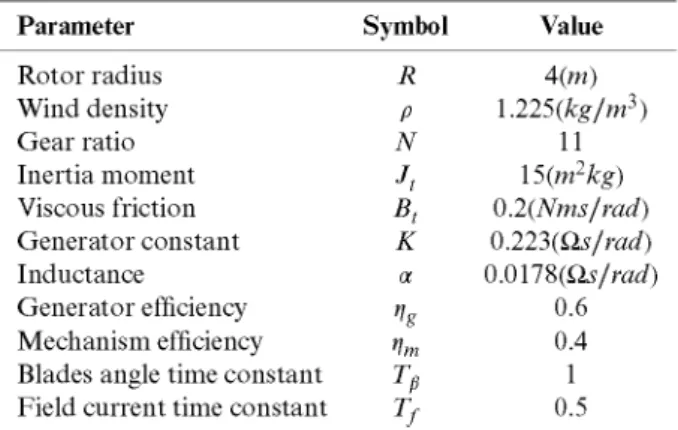
Table II. Wind turbine parameters.

Parameter Symbol Value

Rotor radius Wind density Gear ratio Inertia moment Viscous friction Generator constant Inductance

Generator efficiency Mechanism efficiency Blades angle time constant Field current time constant

R P N

J, B, K a

1g

tfm

Tfi

Tf

4(m) \.225(kg/m3)

11

\5(m2kg)

0.2(Nms/rad)

0.223(Os /rod) 0.017'8(Os/W)

0.6 0.4 1 0.5

Table III. Wind turbine operating point.

Variable Equation

Wind speed vw W.55(m/s)

Electrical line resistance RL 4(ii)

Field current L 2(A) Blades angle fi 7(°)

Rotor angular speed cor 32.24(rad/s)

Generated power Pg 1791.%(W)

If{s)

\ + TfS

W

The order of the wind turbine subsystems dynam-ics is taken into account as follows: the first order drive-train mechanism dynamic, the second order blades angle dynamic and the first order field current dynamics. Thus, the overall system dynamics for both outputs, rotor angular speed a>r and generated power P is fourth order.

Table II summarizes the wind turbine parameters and Table III describes one of the possible operating points proposed for the wind turbine nominal operation, in which we have linearized the nonlinear wind turbine model to obtain the proposed linear controllers.

We have modelled the hardware requirements of the actuators in equations 1 and 2, and the sensors are sup-posed to be ideal, so they have not been modelled. We have considered the wind speed vw as non-manipulated measurable input (measurable disturbance), but we have not modelled it since the results are developed in front of step disturbances in the wind speed, in order to clearly show the proposed controllers behaviour.

III. MULTIVARIABLE MODELLING A N D CONTROL M E T H O D O L O G Y

and incremental state models of any linear system, or at least linearized ones. Once the state model is obtained, we can apply the appropriate controller and observer to achieve the control objectives.

3.1 Multivariable discrete state model

Given a multivariable discrete system with/) manip-ulated inputs u e W, r non-manipmanip-ulated measurable inputs (measurable disturbances) d e W and q out-puts y e 9l?, where q < p, its model in difference

equations can be obtained by input-output identifica-tion. Affine terms can be used to avoid using incremental values around operating point:

yt(k + 1) = ai0 + anyt(k) + ai2yt(k - 1) + • • • p

+ ajn.ytik - «,• + 1) + Y, (byiuj(k)+ 7 = 1

+bij2Uj(k - ! ) + ••• + by„.Uj(k - «,• + 1))

+ £(*rftfi4(*0 + W*/(*

-

) +

-1=1

+bdiinA(k - « , • + !)

(3)

For each output, the difference equation can be transformed in a discrete state model with affine terms:

xt{k) e W>

xt(k+ 1) =

ai0 ' ai\

ai0 ' ail

_ ai0 ' aini _

+

+

+

' an 1 •• • 0

ai2 0 ••. 0

; ; ••. i

_«»,, 0 - - - 0

^ r l l bm • • • bipi

bj\2 bi22 • • • bip2

_ "i\nf "i2nf ' ' ' "ipnf

xt{k)

ux{k)

u2ik)

_ up(k) _

bdm bdm ' ' ' bdiri 1 bdil2 bdi22 ' ' ' bdir2

bdi\nt I 'di2 ij ' ' ' dir ni -1

'dx{k)~ d2{k)

_drQ

0.

(4)

yi(k) = am+[l 0 ••• 0]*,(*:) Discrete model based on input-output identification

xt(k +l) = axi + AtXiik) + Btu(k) + Bdid(k)

yt(k) = ai0 + CiXiik) (5)

where axi e Wn'xl\ At e 9t("<x"<), Bt e Jl<>w), £A e

9l(n<xr) and Q e SR(lx^.

Grouping the whole multivariate system in an unique model, we obtain:

+

+

xq(k+\)

Ax 0 ••• 0

0 A2 ••• 0

0 0 • • • A„

2x2

+

xq

' xx(k) x2(k)

xq{k)

+

B,

B,

uxik) u2ik)

uJk)

+

no

+

ym

y2(k)

yq(k)

c

o ••• o

0 0 • • • C„

B

dx(k) d2{k)

dr(k)

(6)

a20

•lq0

+

x\(k) x2(k)

Xg(k)

which can be represented as follows:

x(k + 1) = ax + Ax(k) + Bu(k) + Bdd(k)

yik) = ay+ Cxik) (7)

where the n Ml + «9 + + K, ax jj(«xi) ^ e ^("X"), B e 9t(nx^, ^ e Wnxr\ ay e 9l(<?xl),

C e 9t(?x") and some of the parameters ain,,biln,,... bt „., bdiXn,... bdim are not null. The system has been identified using input-output data, then the obtained state model will be controllable and observable.

Note that the d inputs are non-manipulated ones and it cannot be used in state feedback, but that d inputs and Bd matrix can be considered in the observer formu-lation, thus improving the state estimation.

3.2 State controller and observer

In order to calculate the coefficients of the state feedback controller K, any state control design

methodology can be applied. Discrete LQR [31,32]

method is chosen, which allows optimal control weight-ing the dynamic response and the control action. The advantages of using discrete LQR is that this algorithm designs a controller matrix for the optimal state control. Also, discrete LQR algorithm is an easy method for the controllers design and it is possible to be applied with different state models.

In LQR method, since the target state is not null, the goal is to minimize the cost index / , which necessitates the tuning of state Q and input R weighting matrices, and the knowledge of state and input references, xr and ur.

J=^[(x(k)-xr)TQ(x(k)-xr)+

k=0

+(u(k) — ur) R(u(k) — ur)\

(8)

However, from the point of view of real applications, the aim is to achieve a desired output value yr, so we pro-pose a systematic method whose objective is to obtain the state and input references, xr and ur, for a desired output reference jr.

Recalling the system state equation described in (7), the objective is to achieve yr. Thus, the variables x(k), u(k) and y{k) are considered to be in steady state (xr, ur and yr). Then it must fulfil:

xr = ax + Axr + Bur + Bdd(k)

Rearranging:

{A — I)xr + Bur = —ax — Bddik) Cxr = yr — o.y

(9)

matrix form:

(A-I)B'

C 0 ur =

-ax - Bdd{k) yr - ay

Solving for xr and ur:

xr ur

(A-I)B C 0

— i

-ax - Bdd{k) yr - ay

and the control action becomes:

uik) = K(xr — xik)) + ur

(10)

(11)

(12)

On the other hand, since the state xik) is not directly accessible, a state observer is required. We choose an optimal observer [30].

Recalling the system given by (7):

x(k + 1) = ax + Axik) + Bu(k) + Bdd(k) yik) = ay+ Cxik)

the observer is formulated as follows:

xe(k + 1) = ax + Axe(k) + Bu(k) + Bdd(k)+ + H(y(k)-(ay + Cxe(k)))

(13)

where H e9Hnx*\

The optimal observer [30] solves the problem of calculating a matrix H which minimizes the cost index / :

J(H) = aT(A- HC) (A - HC)1 a (14)

V « e 9 t "

It is verified in [30] that for any value of a, it fulfills:

H = ACT(CCT)~l (15)

As the matrix C is defined in this particular state representation, it holds that:

CCT = 1

so that:

H = ACT

(16)

(17)

The separation principle holds between optimal observer and control design.

3.3 Incremental state model

As commented before, the proposed method to obtain the state and inputs references, xr and ur (11), can produce steady state errors in presence of modelling errors. This problem can be solved by incremental state model [30].

Applying the discrete state model described in (7), at the previous sample (k-l), we get:

x{k) = ax + Axik - 1) + Bu(k - 1) + Bdd{k - 1) yik - 1) = ay + Cxik — 1)

(18)

x(k+l)- xik) = A ixik) -x(k-l)) +

+ Biuik) - uik - 1)) + Bd idik) - dik - 1)) (19) yik) - yik - \) = C ixik)-xik-\))

where the affme terms are cancelled. Defining the incre-mental state Ax, the increincre-mental manipulated input AM and the incremental non-manipulated measurable input Ad as follows:

Axik) = xik) - xik - I) Auik) = uik) -uik-I) Adik) = dik) - dik - 1)

Substituting (20) into (19), we obtain:

Axik + 1) = A Axik) + BAuik) + BdAd{k) yik) = yik- 1) + C A x i k )

(20)

(21)

New/) states are introduced to complete the formulation, verifying that:

yik+\)= yik) + CAxik + 1) =

= yik) + C (AAxik) + BAuik) + BdAdik)) (22)

We define a new expanded incremental state vector xa 9l(?+n), obtaining the new state model as follows:

xaik) yik) Axik)

+

CB B

I CA 0 A CBd

B,

yik) Axik)

Adik)

+

(23) Auik) +

yik) = [10]

In matrix notation, the expanded state model becomes:

xaik + 1) = Aaxaik) + BaAuik) + BdaAdik) yik)

Axik)

yik) = Caxaik) (24)

Subtracting (18) from (7), we get:

If the control objective is to approach a steady state outputyr, this is equivalent to achieve the reference expanded state in incremental model [30]:

yr Ax,

It should be noted that the reference expanded state comes naturally without the necessity of performing any calculations. Then the control action is described as:

Au(k) = K (xar - xa(k)) =

yr] _ \ y(k)

0 Ax{k)

= [

y

A

uik) = uik- 1) + Au(k)

(25)

(26)

If the feedback system is stable and the steady state is approached, the following conditions are fulfilled:

lim Au(k) = 0, lim Ax(k) = 0

and thus

lim Ky(yr-yik)) =0

So, if K is of rank q, it verifies that:

lim yik) = yr

therefore, the controlled system has zero steady state error.

Note that control action (26) is calculated in incre-mental form (25), which is equivalent to apply an integral control action.

On the other hand, we suppose that the output yik) is measurable, but the incremental state Ax{k) is not

directly accessible, then a state observer is required. The estimated incremental state can be obtained by the state observer described in previous Section 3.2:

Axeik) = xeik) - xe(k - 1) (27)

or directly by the incremental state observer [30], which is formulated as follows:

Axe(k + 1) = AAxe(k) + BAu(k)+

+ BdAd(k) + H (y(k) -y{k-\)- CAxe{k)) (28)

where H e yi1-"^ coefficients are obtained by optimal state observer design [30], as described in (17).

Finally, the expanded estimated state is obtained as follows:

xaik) yik)

Axeik) (29)

IV. P R O P O S E D CONTROLLERS A N D RESULTS ANALYSIS

In this section, we apply the proposed linear control methods to the nonlinear wind turbine model described in Section II, comparing the performances of the mental state model control with those of the non incre-mental one, in order to choose the most adequate solution.

That wind turbine model works in continuous time, but the controller has been developed in discrete time, so a sampler and zero order holding device have been added to the model. All system variables are supposed to be ideally measured.

In order to obtain the proposed linear controllers, we have identified, by the least squares method, the fol-lowing linearized system of the nonlinear wind turbine model, around the operating point defined in Table III, supposing the proposed sampling time is T = 0.05s:

mrik+ 1) = 0.0012 + 2.7318mr

ik)-- 2Al52mrik - 1) + 0.6228®r(A: - 2)+

+ 0.0604®r(A: - 3) + 0A094vwik) - 0.1A01vwik - 1) + 0.3054vw(A: - 2)+

+ 0.0268vw(A: - 3) - 0.00005/?r

(A:)-- 0.0002/?r(A: - 1) - 0.000\flr(k 2 ) -- 0.000007/?r(A: - 3) - 0.0363//r

(A:)-- 0.0013//r(Jfc - 1) + 0.0336//r(A: - 2)+

+ 0.0025//r(A: - 3)

(30)

Pgik+l) = -0.7204 + 2.1484Pg

ik)-- 0.1196Pgik - 1) - 0.9041 Pgik - 2)+

+ 0.5351 Pgik - 3) + 13.0373vw

(A:)-- 15.9819vw(A:- 1) -4.5794vw(A:-2)+

+ 7.5706vw(A: - 3) -

0.0014fl.(Jfc)-- 0.0065/?r(A: - 1) - 0.0051/?r(A: 2 )

-- 0.001 \flr(k - 3) + 169.3539//r

(A:)-- 2\2.153Ifrik - 1) - 57.8343//r(A: - 2)+

4.1 Discrete state model (31) From the input/output identified model (equations 30 and 31) and following the methodology described in previous Section 3.1, the wind turbine discrete state model (7) is obtained:

x(k + 1) = ax + Axik) + Bu(k) + Bdd(k) yik) = ay+ Cxik)

where:

x(k)

yik)--B:

9t8

cor(k) Pg(k)

0.0034 -0.0030 0.0008 0.0001 -1.5478 0.5617 0.6518 -0.3859 -0.00005 -0.0002 -0.0001 -0.000007 -0.0014 -0.0065 -0.0051 -0.0011 , uik) ,B, 0r(k) '/,(*> 0.4094 -0.7407 0.3054 0.0268 13.0373 -15.9819 -4.5794 7.5706

, d(k) = vwik)

-0.0363 -0.0013 0.0336 0.0025 169.3539 -212.7530 -57.8343 101.6462 A =

2.7318 1 0 0 -2.4152 0 1 0

C = 0.6228 0.0604 0 0 0 0 0.0012 -0.7204

1 0 0 0 0 0 0 0 0 0 0 0 1 0 0 0 0 0 1 0 0 0 0 0 0 0 0 0 0 0 0 0 0 0

0 0 0 0 2.1484

0 0 0 0 0 0 0 0 0 0 0 0 1 0 0 -0.7796 0 1 0 -0.9047 0 0 1 0.5357 0 0 0

Note that wind speed vw is a non-manipulated input. As described in Section 3.1, it cannot be used in state feedback, but vw input and Bd matrix can be considered in the observer.

The controller algorithm is designed by the dis-crete LQR method, using the following positive definite weighting matrices:

Q = diag([l 1 1 1 1 1 1 1 ] )

R = diag([\ 1])

We obtain the state and input references as described in equation (11): xr ur iA-I)B C 0 — 1

-ax - Bddik) yr - ay

As described in equation (12), the control action becomes:

uik) = K{xr — x(k)) + ur

with:

[-79.5628 -77.8970 -76.0858 -74.136 ~ [ -0.0002 -0.0001 -0.00004 0.00005 -2.9806 -2.9068 -2.8207 -2.7252"

0.0073 0.0020 -0.0024 -0.0006

And the state observer, defined in equation (13) is:

xeik + 1) = ax + Axeik) + Bu(k) + Bddik)+ + H [yik) — ay — Cxeik))

with: H 2.7318 -2.4152 0.6228 0.0604 0 0 0 0 0 0 0 0 2.1484 -0.7796 -0.9047 0.5357

4.2 Incremental state model

Wind turbine incremental state model equations are described by equation (24):

xa(k + 1) = Aaxaik) + BaAuik) + BdaAdik) yik) = Caxaik)

where:

xaik) =

uik) = yik) Axik)

$rik) ' Ifik) Axik)e%\AaeViWxW

,yik) =

, d(k) = vJk) mrik) P.ik)

B„eK 10x2 B da 91

10x1

The controller algorithm is designed by the dis-crete LQR method, using the following positive definite weighting matrices:

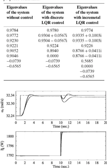
Table IV. Eigenvalues of the system with and without the proposed controllers.

Q = R =

( [ 1 1 1 1 1 1 1 1 1 1 ] )

( [ 1 1 ] )

As described in equations (25) and (26), the control action is:

Au(k) = K (x, xa(k))

u(k) = u(k- 1) + Au(k)

with:

[-0.9048 -0.0209 -721.0133 -666.949 [-0.0001 0.0025 -0.0636 -0.0590

-613.4391 -561.5192 -0.7790 -0.0545 -0.0501 0.0141 -0.5897 -0.3961 -0.2050"

0.0075 0.0018 0.0020

And the state observer, described in equations (28) and (29), is:

Axe(k + 1) = AAxe(k) + BAu{k) + BdAd(k)+

+ H{y{k)-y{k-\)-CAxe{k))

x (k)_\ yik)

aeK ' [ Axe(k)

with the same H matrix obtained in previous Section 4.1.

4.3 Results and analysis

In all the figures presented in this section, the incre-mental state model response is shown in continuous line and the non incremental state model response in dot-ted line. If reference signal is represendot-ted, it is shown in dashed line.

Table IV shows the eigenvalues of the system with and without the proposed controllers. It can be observed that the eigenvalues of the system without control, the system controlled by discrete LQR and the system con-trolled by incremental LQR are very similar. This means that the controlled systems have similar dynamics. How-ever, the objective of the proposed controllers is not mod-ifying the dynamic behaviour of the wind turbine, which is considered adequate, but to guarantee the disturbances rejection.

Fig. 4 shows the dynamic behaviour of the wind tur-bine model, controlled by discrete and incremental LQR algorithms, subjected to changes in the reference signal of rotor angular speed a>r and generated power P

Eigenvalues of the system without control

0.9784 0.9772 0.9230 0.9221 0.9052 0.9046 -0.0739 -0.6565

Eigenvalues of the system with discrete LQR control

0.9780 0.9304 + 0.0567i 0.9304 - 0.0567i

0.9224 0.8940 0.0000 -0.0739 -0.6565

Eigenvalues of the system with incremetal

LQR control 0.9774 0.9335+ 0.1003i 0.9335-0.1003i

0.9226 0.8766 + 0.041 li 0.8766 -0.041H

0.5685 0.0000 -0.0739 -0.6565

1800

1796

1792

0 2 4 6 8 10 12 14 16 18 20 Time (sec.)

Fig. 4. Rotor angular speed wr and generated power P„ responses to changes in references signals.

It can be observed that, both controlled responses present similar dynamic behaviour. However, even with the adjustment method of state and input references xr and ur, the controlled system by discrete LQR presents small steady state errors, because of modelling errors, which do not appear in the controlled system by incre-mental state model.

In order to compare the performances of the con-trollers in presence of disturbances, changes in wind speed vw and line resistance Rt are applied. Fig. 5 shows the dynamic behaviour of the wind turbine model, con-trolled by discrete and incremental LQR algorithms, sub-jected to changes in the reference signal of rotor angular

speed a>r and generated power P Moreover, it is sub-jected to step disturbances in wind speed from vw =

1804

g- 1800

PS° 1796 1792

0

20 25 30 Time (sec.)

-— F="

10 15 20 25 30

Time (sec.) 35 40 45 50

Fig. 5. Rotor angular speed wr and generated power P

responses to changes in references signals and disturbances.

2200

2000

1800

1600

10 15 20 25 30 Time (sec.)

35 40 45 50

1

n r

10 15 20 25 30 Time (sec.)

35 40 45 50

Fig. 7. Rotor angular speed wr and generated power P

responses to changes in references signals and excessive disturbances.

20 25 30 Time (sec.)

Fig. 6. Rotor angular speed wr and generated power P

observation errors.

from Rt = 4.00Q. to Rt = 4.01Qatt = 35s. Fig. 6 shows the Observation Error (OE).

It can be observed that, even both controllers pro-duces similar dynamic behaviour, the controlled system by discrete LQR presents steady state errors. On the other hand, incremental state feedback method produces zero steady state error even in presence of modelling errors, nonlinearities and unmodelled disturbances.

It can be checked that the optimal state observer produces fast convergence to zero observation error and, because of considering vw input and Bd matrix in the state observer formulation, the observation error pro-duced by wind speed vw disturbance in t = 10s has low amplitude. The observation error produced with the non incremental state model presents a small steady state error making impossible the complete convergence

between the estimated state and the real one. Incremen-tal state model presents zero steady state error also in the observation error.

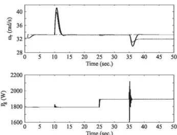
In order to compare the performances of the con-trollers in the above rated zone and in presence of large disturbances, excessive changes in wind speed vw and line resistance Rt are applied. Fig. 7 shows the dynamic behaviour of the wind turbine model, controlled by dis-crete and incremental LQR algorithms, subjected to changes in the reference signal of rotor angular speed G)r and generated power P Moreover, it is subjected to step disturbances in wind speed from vw = 10.55m/s to vw = 13.00m/s at t = 10s and line resistance from R, = 4.00S2 to R, = 4.50S2 at t = 35s.

It can be seen that both state models control algo-rithms can provide stability in the full range of the above rated zone, but the nonlinearities of the model have changed the dynamic behaviour of the controlled system. Also, the steady state error of the controlled system by discrete LQR is too high for a good nominal operation, so zero steady state error must be obtained and it has been got by the incremental state model control.

V. CONCLUSIONS

In this paper, we have proposed a multivariable opti-mal control of wind turbines using a new methodology based on incremental state model, with a LQR control and an optimal observer.

• First, control action in incremental state model is equivalent to introduce an integral action, cancelling the steady state errors produced by the n o n incre-mental formulation.

• Second, in the classical L Q R control, the reference state should be calculated, while in the incremen-tal L Q R control, the reference state is directly the o u t p u t reference with a null reference for the state increase.

The application of the proposed linear controller to the simulated w i n d turbine nonlinear model has shown that incremental L Q R control presents a good transient response and zero steady state error, even in presence of modelling errors, nonlinearities and disturbances.

We propose as future work, to design an exten-sion of the proposed control method using a non-linear a p p r o a c h by the T-S fuzzy model. Wind turbines are non-linear systems with strong nonlinearities in the slow wind zone, thus a non-linear a p p r o a c h of the incremen-tal state control method based in T-S fuzzy models could obtain better results in the full operation range of the wind turbine, with the same advantages of the proposed linear controller.

VI. APPENDIX

6.1. Nomenclature and list of abbreviations

fir

RL

CO.

CP C, P

u r d q y X n

ax

A B Bd

ay

C K J Q R

ur yr H T t

LQR PI PID QFT CART 3 MSISO MIMO DEMM DMC RGPC OE T-S

Table A l . Nomenclature. Blades angle reference

Field current reference Wind speed

Electrical line resistance Rotor angular speed Generated power Blades angle Field current Power coefficient Mechanical coefficient

Number of system manipulated inputs System manipulated inputs

Number of system measurable disturbances System measurable disturbances

Number of system outputs System outputs

System states

Number of system states State affine terms matrix State dynamic matrix Input dynamic matrix Disturbance dynamic matrix Output affine terms matrix Output matrix

State controller matrix Cost index function State weighting matrix Input weighting matrix State reference Input reference Output reference State observer matrix Sampling time Time

Table A2. List of abbreviations. Linear Quadratic Regulator Proportional Integral

Proportional Integral Derivative Quantitative Feedback Theory

Controls Advanced Research Turbine 3-bladed multiple single-input single-output

multiple-input multiple-output Difference Equation Matrix Model Dynamic Matrix Control

Recursive Generalized Predictive Control Observation Error