Optimal control of a ball and beam nonlinear model based on Takagi-Sugeno fuzzy model

Optimal Control of a Ball and Beam N onlinear

Model Based on Takagi-Sugeno Fuzzy Model

José Miguel Adánez Basil Mohammed Al-Hadithi Agustín Jiménez

Abstract. In this work, an improved approach for Takagi-Sugeno sys­ tem identification is used. Linear Quadratic Regulator is applied for an optimal state feedback. Duality theorem and Linear Quadratic Regula­ tor is applied for an optimal state estimation. Simulation results over the ball and beam nonlinear model show a stable closed loop in the full range and good transient response.

1 Introduction

The ball and beam system [1] is a classical mechanical system with two degrees of freedom. The beam rotates, driven by a torque at the center of rotation. The ball rolls freely along the beam and in contact with the beam. Despite its mechanical simplicity, the ball and beam system presents significant challenges

from the point of view of automation; the system is nonlinear and unstable. The ball and beam is a common didactical plant in many control laboratories around the world [2], as it is very nonlinear, unstable, which means that it is difficult to control, and can be a benchmark for testing several advanced control techniques [3].

Takagi-Sugeno (T-S) fuzzy model [4] has been an important tool for the modelling and control of nonlinear systems, since it builds the full nonlinear model by a linear model at each fuzzy rule and the fuzzy interpolation among them. Moreover, the T-S fuzzy identification allows the identification of all the fuzzy parameters of the full nonlinear system minimizing a global error index.

Optimal control has been a significant method for the controllers design. Linear Quadratic Regulator [5], is an optimal control design method for state space linear models which allows the minimization of a cost function in which state dynamics and control action are weighted.

One of t h e most i m p o r t a n t problems in s t a t e space feedback is t h a t usually t h e states are not directly accessible, since not all t h e s t a t e variables are mea-surable. For this propose, s t a t e observers [6], can create a surrogate s t a t e vector, which t e n d s asymptotically t o t h e real s t a t e vector and can be used for s t a t e feedback.

T h e duality theorem [6] allows t h e design of an s t a t e observer m a t r i x with t h e same techniques for an s t a t e feedback controller, including t h e L Q R m e t h o d [5]. For t h a t propose a dual system can be built from t h e s t a t e space model, and t h e duality theorem says t h a t a controller designed in t h e dual system is equivalent t o an observer designed for t h e s t a t e space model.

T h e rest of t h e work is organized as follows. Section 2 describes ball and b e a m nonlinear model. T h e fuzzy T-S model and t h e fuzzy identification m e t h o d are described in Sect. 3. O p t i m a l s t a t e controller and optimal s t a t e observer designs are described in Sect. 4. In Sect. 5, t h e proposed fuzzy optimal controller is applied t o t h e ball and b e a m nonlinear model and t h e results are obtained and discussed.

2 Ball a n d B e a m Nonlinear Model

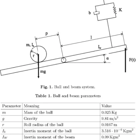
In this work, we use t h e A M I R A BW500 ball and b e a m model (Fig. 1) [1]. T h e ball position p, considered as system o u t p u t , is supposed t o be measured by a camera, therefore t h e discrete sample time is supposed t o be large. T h e b e a m angle a, considered as measurable internal variable, is supposed t o be measured by an incremental encoder. T h e system input F is supposed t o be a force produced by a DC motor, which causes t h e b e a m t o r o t a t e around its center.

T h e nonlinear differential equations of t h e ball and b e a m model [1], used for t h e simulation model, are:

m -\—r- \ p + (mr + _/&) —a — mpa = m<;sin(a) (1)

(mp2 +Ib + Iw) a + (2mpp + bl2) a + Kl2a+

1 .. (2)

(mr + lb) — p — mgp cos(a) = i*7cos(a)

where p is t h e position of t h e ball, a is t h e angle of t h e b e a m and F is t h e force of t h e drive mechanics. Table 1 summarizes t h e p a r a m e t e r s of t h e model and its values.

In this model, some restrictions from t h e real A M I R A BW500 ball and b e a m model [1] have t o be added. T h e ball position p has t o be contained in [—0.4,0.4] m, t h e b e a m angle a has t o be contained in [—0.69,0.69] rad and t h e input force F has t o be contained in [—5, 5] N.

Fig. 1. Ball and beam system.

Table 1. Ball and beam parameters

Parameter

m

9 r

lb

Iw b

K I

Meaning

Mass of the ball

Gravity

Roll radius of the ball

Inertia moment of the ball Inertia moment of the beam

Friction coefficient of the drive mechanics

Stiffness of the drive mechanics Radius of force application

Value

0.025 Kg

9.81 m / s2

0.0167m

3 . 5 1 6 - l O ^ K g m2

0.09 Kgm2

l.ONs/m

0.001 N / m 0.49 m

3 Fuzzy Takagi-Sugeno Model and System Identification

3 . 1 F u z z y T - S M o d e l

Nonlinear systems c a n b e modelled b y T-S model, supposing known a set of measurable nonlinear variables [zi(k), Z2(k),..., zm(k)] of t h e system. By choos-ing [ri, r 2 , . . . , rm] number of fuzzy sets for these variables, a monovariable fuzzy system can b e defined as follows:

S{ii-im). I f Zi(kj i g Mh a n d _ a n d Zm(kj i g Mi^ t h e n.

y(k) = at-im) + at-im)y{k -!) + ••• + a^-A^y{k - n) (3)

In each rule, we can transform the difference Eq. (3) to state model with affine term as follows:

S(h-im). if Zl(fy i s Mn a n d _ a n d Zm(kj i s Mi™ t h e n.

x(k) e 9 T

x(k + 1)

(ii—ir. (i1...ir.

(ii-ir.

( i i . . . i „

( i i . . . i „

• 4

"

1 ••• 0

o '•. o

: : •• 1 x{k)

b(il...im)

l(il--im)

u{k)

){k) = 4i l ," ' ") + [l0---0]x(jfe)

This means

S{il-im). Jf ^(fc) i g Mj l a n d _ a n d Zm(J^ i g Mir, t h e n.

x(jfe + 1) = o f1- ' " ' + ^ ' " ^ ( A ; ) + B^-A^u{k)

y(k)=a^-i^ + Cx(k)

(4)

(5)

3.2 Estimation of T-S Model Parameters

The identification method of T-S fuzzy models [4] is based on the estimation of the fuzzy system parameters minimizing a quadratic performance index. The traditional T-S identification method [4] fails if the membership functions of the fuzzy rules are overlapped triangular in shape, since the T-S matrix is not of full rank and then it is not invertible [7]. Thus, in [7] was proposed a generalized T-S identification, using a parameters weighting method.

The fuzzy estimation of the output becomes:

7*1 rm

*1=1 im=l

7( i i .

/?

-

(Hn..,

)(k)) [ot-

+ ot-

y(k - 1)

]y{k - n) + b((1-im)u{k - ! ) + ••• + b^-im)u{k - n)

(6)

where

/ ?( i l-i m )( * ( i i . . . im) W )

M i i i ( z i ) •• • ferritin \^m)

We have supposed to have a set of input/output system samples and a first affine linear parameters estimation:

/ = [ a g a ? . . . a ° 6 ? . . . 6 ° ]

These parameters could be obtained by a classical input/output identification of the data, for example with least squares method. This first approximation can be utilized as reference parameters for all the subsystems. Then, the fuzzy model parameters can be obtained minimizing:

j = Y

(y(k)-y(k)f+l

J2

fc=i jm= l j = 0

p°i -p ( * l - . - * m )

(9)

= \\Y-XP\\2+^\\P0

Pf =

~

x~

J

.

p = \\Ya ~ XaP\\

where Y are the output data, X are the input/output fuzzy data, PQ are the linear estimated parameters repeated as many times as the number of fuzzy rules (Po = \po,Po, • • • >Po\), a n (i P a r e the fuzzy T-S model parameters. The 7 factor

represents the degree of confidence of the linear estimated parameters, and it must be tuned by try and error. It should be noted that the matrix Xa is of full

rank, which solves the problem where the traditional T-S identification method fails. Thus, the vector P can be computed as:

P — \XaXa) XaYa (10)

4 Fuzzy Controller a n d Observer Design

In order to calculate the coefficients of the state feedback controller, discrete LQR [5] method is chosen, which allows optimal control weighting the dynamic response and the control action.

In LQR method, the goal is to minimize the cost index J:

0 0

J = \ (x(k) — xr) Q (x(k) — xr) + (u(k) — ur) R (u(k) — ur) fc=0

(11)

LQR method is completely optimal for linear systems, however, in the case of nonlinear systems, it is complex to propose the minimization of any objective function for the global system. In order to solve this problem, we suggest mini-mizing the cost of each fuzzy rule instead of the global cost. The solution will be a suboptimal one but with the great advantage of being easy to calculate. With this method, the global stability is not guaranteed, which needs to be analyzed a posteriori, although gaining in return a balance between static and dynamic behavior of the system with admissible control actions.

The state observer [6] is a parallel dynamic system with a correction term that approximates the estimated state to the real one:

xe(k + 1) = ax + Axe(k) + Bu(k) + H (y(k) - ye(k))

ye(k) = ay + Cxe(k)

The estimation error is:

e(k + 1) = x(k + 1) - xe(k + 1) = (ax + Ax(k) + Bu{k))

- (ax + Axe(k) + Bu{k) + H(y(k) - (ay + Cxe{k))))

which can be rewritten as follows:

e{k + l) = {A-HC)e{k) (14)

The duality theorem [6] states that the design of a state observer is equivalent to designing a state feedback controller using some transformations in the state matrices. Based on the linear discrete system described as:

(15)

(16) x(k + 1) = Ax(k) + Bu{k)

y{k) = Cx{k)

The corresponding dual system becomes:

xd(k + 1) = Adxd(k) + Bdu(k)

yd(k) = Cdxd(k)

where:

Ad = At

Bd = Cl (17)

Cd = Bl

Therefore, it is possible to calculate a control matrix for the dual system Kd

equivalent to the observation matrix for the original system H:

H = Kd (18)

In this way, is possible calculate the observation matrix H, obtaining the controller matrix for the dual system Kd by any state controller design method

in the dual system. In this discrete LQR [5] is proposed, obtaining the H observer matrix from the dual system matrices Ad = A1 and Bd = C', and

the weighing matrices Qd and Rd, minimizing the following index cost:

oo

J = Y. [xd(kYQdxd(k) + u(kYRdu(k)] (19)

fc=0

5 R e s u l t s

In this section, we apply the proposed fuzzy optimal controller to the ball and

beam nonlinear model described in Sect. 2. The ball and beam model works in

As first step, a linear identification of the system has been made by least squares method, obtaining a first affine linear parameters estimation:

p(k) = 0 + 3.92p(k - 1) - 5.75p(k - 2) + 3.75p(k - 3) - 0.92p(k - 4) - 0.0001F(k - 1) + 0.0001F(k - 2) + 0.0001F(k - 3) - 0.0001F(k - 4)

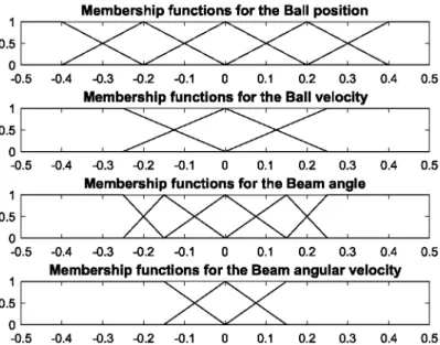
For a T-S model identification of the system, an iterative adjustment of the membership functions of the fuzzy rules and the weighting factor 7 have been made, adjusting by try and error the fuzzy membership functions defined in Fig. 2 and the weighting factor 7 = 3.7 • 10~6, obtaining an identification error of 1.616910-11.

With the generalized T-S identification method and Eq. (4), a fuzzy T-S state matrices of the system has been obtained:

5(1,1,1,1). I f ^ i g Ml a n d p ^ i g Ml a n d a(^ i g Ml a n d Q,^) i g Ml t h e n.

^ l , ! , ! , ! ) _ _{= 1(T}5 [0.3146 -0.4620 0.3014 -0.0737]

^4(1,1,1,1)

3.9181 1 0 0 -5.7542 0 1 0

3.7543 0 0 1 -0.918100 0

5(1,1,1,1) = 1 Q- 3 [_o.0578 0.1418 0.1160 -0.0544]'

a(i, 1,1,1) = g.0285 • 1 0 "7

Cr(i,i,i,D= [10 0 0]

Thus, the controller matrix K is designed in each rule by discrete LQR [5] algorithm, using the system matrices A and B, and the positive definite weighting matrices Q = I and R = 1. Obtaining the fuzzy controller matrix:

5(l,l,l,l). If^ i g Ml a n d p ^ i g Ml a n d a(^ i g Ml a n d Q,^) i g ^ 1 t h e n. ^(1,1,1,1) = 1 0 3 [2.9586 2.5483 2.1733 1.8322]

The observer algorithm is designed in each rule by duality theorem [6] and

discrete LQR algorithm [5], using the dual system matrices Ad = A1 and Bd =

C', and the positive definite weighting matrices Qd = I and Rd = 1. Obtaining the fuzzy observer matrix by the Eq. (18):

5(1,1,1,1). U p ^ i s Mi a n d p ^ i s Mi a n d a(j^ i s Mi a n d a(j^ i s Mi t h e n.

^(1,1,1,1) = [2.7955 -4.9873 3.4842 -0.8789]*

1

0.5

0.5 -0.4 -0.3 -0.2 -0.1 0 0.1 0.2 0.3 0.4 0.5 Membership functions for the Ball velocity

1

0.5

0.5 -0.4 -0.3 -0.2 -0.1 0 0.1 0.2 0.3 0.4 0.5 Membership functions for the Beam angle

0.5 -0.4 -0.3 -0.2 -0.1 0 0.1 0.2 0.3 0.4 0.5 Membership functions for the Beam angular velocity

0.5

-0.5 -0.4 -0.3 -0.2 -0.1 0 0.1 0.2 0.3 0.4 0.5

Fig. 2. Membership functions of the fuzzy sets.

10 15 20 25 30 35 40 45 50 Time (sec.)

Fig. 3. Ball position.

0.15

-0.15

0 5 10 15 20 25 30 35 40 45 50

Time (sec.)

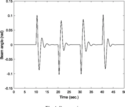
Fig. 4. Beam angle.

x10

10 15 20 25 30 35 40 45

Time (sec.)

F i g . 6. Observation error of ball and beam position.

In Figs. 3, 4 and 5 it can be seen t h a t , t h e system variables are in t h e physical range of t h e ball and beam, and all these variables present s m o o t h and stable transient responses. In Fig. 6 it is shown t h a t t h e observation error is small and t e n d s t o zero. Thus, t h e controlled ball and b e a m model has a stable response in t h e full range of t h e system and presents a good transient response.

6 Conclusion

In this work, we have shown t h e obtained results t h a t a generalized T-S identi-fication m e t h o d and an optimal s t a t e controller and observer designed in each fuzzy rule, applied in a ball and b e a m nonlinear model. T h e fuzzy generalized T-S identification m e t h o d is based on a weighting p a r a m e t e r of t h e previously estimated linear model. T h e optimal controller and observer has been designed in each fuzzy rule, so a suboptimal solution have been found, b u t easy of calcu-late and compute. T h e results show t h a t t h e ball and b e a m controlled nonlinear model has a stable behavior and good transient response on t h e full range of t h e ball and b e a m system.