Application of Vector Spherical Harmonics and Kernel Regression to the Computations of OMM Parameters

Texto completo

(1)The Astronomical Journal, 149:129 (11pp), 2015 April. doi:10.1088/0004-6256/149/4/129. © 2015. The American Astronomical Society. All rights reserved.. APPLICATION OF VECTOR SPHERICAL HARMONICS AND KERNEL REGRESSION TO THE COMPUTATIONS OF OMM PARAMETERS 1. F. J. Marco1, M. J. Martínez2, and J. A. López1 Departamento de Matemáticas, IMAC, Universidad Jaume I. E-12071 Castellón, Spain; marco@mat.uji.es 2 Dep. Matemática Aplicada, IUMPA, Universidad Politécnica de Valencia, E-46022 Valencia, Spain Received 2013 July 22; accepted 2014 December 14; published 2015 March 16. ABSTRACT The high quality of Hipparcos data in position, proper motion, and parallax has allowed for studies about stellar kinematics with the aim of achieving a better physical understanding of our galaxy, based on accurate calculus of the Ogorodnikov–Milne model (OMM) parameters. The use of discrete least squares is the most common adjustment method, but it may lead to errors mainly because of the inhomogeneous spatial distribution of the data. We present an example of the instability of this method using the case of a function given by a linear combination of Legendre polynomials. These polynomials are basic in the use of vector spherical harmonics, which have been used to compute the OMM parameters by several authors, such as Makarov & Murphy, Mignard & Klioner, and Vityazev & Tsvetkov. To overcome the former problem, we propose the use of a mixed method (see Marco et al.) that includes the extension of the functions of residuals to any point on the celestial sphere. The goal is to be able to work with continuous variables in the calculation of the coefficients of the vector spherical harmonic developments with stability and efficiency. We apply this mixed procedure to the study of the kinematics of the stars in our Galaxy, employing the Hipparcos velocity field data to obtain the OMM parameters. Previously, we tested the method by perturbing the Vectorial Spherical Harmonics model as well as the velocity vector field. Key words: astrometry – methods: data analysis – reference systems 1. INTRODUCTION. are usually estimated using the discrete least squares method (DLS). Moreover, VSH have been widely used in both lines of work and for several sub-objectives. See, in particular, the primary contribution of Mignard & Morando (1990) and their further update of that paper, Mignard & Klioner (2012), within the context of the Hipparcos-FK5 comparison. This issue was also studied by us in Marco et al. (2004), where we truncate the VSH development up to the first order, which is enough to determine the rotational and deformation parameters. We also used VSH in the frame of ICRF in Martinez et al. (2009). Within the context of stellar kinematics, VSH are used by Vityazev & Shustsko (2004, 2005), Vityazev & Tsvetkov (2009, 2011, 2012), and Makarov & Murphy (2007), among others. Vityazev & Tsvetkov (2013) extended this study with stellar velocities from the UCAC4 catalog introducing VSH in a zonal catalog (ZVSF) and in Vityazev & Tsvetkov (2014) in UCAC4, PPMXL, and XPM. The common methodology of all these papers is the choice of a particular mathematical model (VSH) to develop the stellar velocity fields, the identification of the link among the coefficients of the development and the physical parameters included in the Ogorodnikov–MilneModel (OMM), and their subsequent determination using DLS (including some possible modifications taking weights into account). We should first point out that even though we could choose any of the two former frameworks (reference frames and stellar kinematics), in this paper we merely try to determine the OMM parameters using VSH and kernel regression. This choice, though it is not the only one, may vary depending on the data of the considered problem. Other authors using Hipparcos data with a different mathematical model are Dehnen & Binney (1998), Famaey et al. (2005), Mignard (2000), Yuan et al. (2008), Zhu & Jin (2000), and du Mont (1977) for the FK4/FK4 Sup stars and Hanson (1987) for the Lick northern Proper Motion program.. The Hipparcos catalog (ESA 1997; for more details, see Perryman et al. 1997) provided a huge number of astrometrical data that have enhanced different fields of study. One of them consists of the definition of a sustainable reference frame which, at the same time, provides a link between the visible wavelengths in the Hipparcos Celestial Reference Frame (HCRF) and the non-visible wavelengths (radio sources, for instance), which must be referred to the International Celestial Reference Frame (currently the ICRF2). The development of new catalogs, such as Tycho-2, UCAC2, UCAC4, PPMXL, XPM, and others (in visible wavelengths) and LQAC and XMM (in non-visible wavelengths) in addition to the future GAIA catalog, aims to extend and improve the HCRF and ICRF2 frames. Other partial catalogs, such as Rio in Assafin et al. (2013) and that in Zacharias & Zacharias (2014) with a few data sets, aim to increase the number of “reference sources” that are suitable for use in linking both reference frames. A second line of work is the study of the kinematics of the stars in our galaxy, employing Hipparcos, UCAC4, PPMXL, and XPM. On solving both problems, progress has been made using physico-mathematical functional models with increasing complexity (infinitesimal rotations, rotations+deformations, Surface Spherical Harmonics, Fourier–Legendre–Hermite functions, and Vectorial Spherical Harmonics (VSH)), whose parameters may be determined using different procedures. To this aim, it must be assumed that the searched function fulfills the analytical properties that confirm that it has a unique functional development series. In addition, it is commonly assumed that only relatively low order harmonics are included in the series. In our opinion, this assumption is not necessary and can even lead to wrong results, as we see in Section 2.1. In practice, one works with discrete data, and the parameters 1.

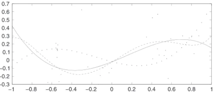
(2) The Astronomical Journal, 149:129 (11pp), 2015 April. Marco, López, & Martínez. At this point, it is necessary to supply explanation of the following. 1. Why a new approximation to the problem may be helpful. 2. What involves this new approximation. From a mathematical point of view, there are two aspects to consider: the mathematical modeling itself (we have already mentioned this issue) and the practical implementation of the model when we use a discrete set of data. The implementation of the model is not a minor topic if we want to obtain trustworthy results. Evidently, we must be very careful when working with a discrete set of points (abscissas) not necessarily homogeneously distributed and with data associated with these points (such as errors in positions, proper motions, radial and tangential velocities, etc.). In addition, the observed values can be affected by random noise. This noise may or not be normal (this question, though very interesting, is out of the scope of this paper). The data are usually processed by means of the classical DLS method. The Gauss–Markov theorem states that this method provides the unbiased estimator of minimum variance if the data are not biased, and provided that the residuals behave as a normal random variable of null mean. If we assume that the data to be fit can be properly mathematically modeled by means of development in a certain functional basis, we must note that the main interesting properties of these functions come from their continuous nature. The spatial distribution of the data may affect the preservation of these good properties when we apply DLS. For example, if the spatial distribution is not homogeneous, orthogonality is not preserved when dealing with the discrete problem, and this influences the reliability of the computed results for the coefficients. We begin the second section with an elementary example of this problem. In this example we see that if we use the DLS, the coefficients are accurately computed only if the order of DLS matches the order of the development in the functional basis. In general, this order of development is not known, so if instability exists, whenever the order of the development is increased the coefficients of lower orders are useful. If higher order harmonics are present in the real problem, even more difficulties arise when we use DLS. On one hand, we cannot choose a priori an arbitrarily high order and, on the other, the higher the order, the more possibilities that an “ill-conditioned” problem appears. Focusing on the problem of the determination of the OMM parameters, it should be emphasized that the discrete method may lead to contradictory results. For instance, in the determination of the OMM parameters carried out by Makarov & Murphy (2007), the authors compute the components of the solar velocity relative to the average motion of the local stars, then these components are removed from the function to adjust, and they carry out a new adjustment. They obtain a surprising s1 - 1 value (denoted as e1-1). The s1 - 1 value results in being related to the vy component of the Sun velocity that had already been subtracted, and it should have been null if orthogonality was preserved. The authors explain this result because the sampled vector harmonics are not independent due to the lack of uniformity in the number density of stars. We raise an alternative method, which we can consider a mixed method (MM) in the following sense.. Figure 1. Example of one of the random samples with 40 points used. We represent the function obtained using DLS (dotted line), the function obtained using CLS (solid line), both of them computed up to the third order, and the real function (dashed line).. regression adjustment methods. This regression can be evaluated on as many points as desired. In particular, it is possible to set a homogeneous network, with equispaced grid points, where we can obtain an estimation of the function that represents the discrete data. So, we have the adjustment of the function or vector field in a set of welldistributed points, which allow us to obtain the coefficients of the function one by one, independently from one another, and up to the desired order. All of this appears as an elementary consequence of the orthogonality, which is verified in the continuous case in which we work. 2. We highlight that we work with the continuous problem and only when necessary do we discretize. We will consider this topic in Section 2.3, including the theoretical justification. The structure of the paper is as follows. In Section 2 we deal with the so-called MM. We note in Section 2.1 the problems that may appear in the DLS method. To this aim, we use 1000 samples of 40 nonhomogeneously distributed points where a selected function is perturbed with a normal with a null mean and standard deviation of 0’25, and we apply DLS to obtain the coefficients for the development in Legendre polynomials of this function. In Section 2.2, we perform the same test employing the MM. Then, in Section 2.3 we describe a brief guideline about the use of smoothing methods as intermediaries in the context of the parametrical adjustments. In Section 2.4 we introduce the treatment of the VSH to obtain a decoupled equation to compute the OMM parameters. This last issue is treated in Section 3 for the case of the Hipparcosstellar velocity field. We conclude Section 2 by noting the advantages of the method in Section 2.5. In Section 3 we present the OMM model and describe how to apply our method to obtain the coefficients of this model. In Section 3.1, we carry out 2 simulations of the method with 1000 samples of 42,763 points. First, a systematic component of the form å l2=1å lm=-l éë tl, m Tl, m + sl, m Sl, m ùû with an amplitude of 200*N(0,1) km s−1 kpc−1 is introduced into the model proper motions. Second, a large random component with a perturbation of 20*N(0,1) km s−1 is introduced into the model tangential velocities. Finally, in Section 3.2 we compute the OMM parameters from the tangential velocities of 42,763 selected Hipparcos stars and compare the values obtained by us with those of other authors. To end the paper, there is a summary of results and conclusions as well as possible improvements, followed by three appendices where we describe the Local Polynomial Kernel Smoothing Method, provide an extension of the. 1. Given the discrete data, we can obtain an adjustment in the whole domain of the definition. We remark that we are not dealing with interpolation methods, but with smoothing 2.

(3) The Astronomical Journal, 149:129 (11pp), 2015 April. Marco, López, & Martínez. Table 1 Results for the Mean and Standard Deviation of the Coefficients Obtained using 1000 Samples of 40 Points, for DLS of the Order of 0, 1, 2, 3, 4, and 5 and for CLS (Continuous Least Squares Method) Order/Coef 0 1 2 3 4 5 5 (CLS) 5 (True). a0. a1. a2. a3. a4. a5. 0.16 ± 0.11 0.15 ± 0.09 0.09 ± 0.06 0.09 ± 0.06 0.09 ± 0.06 0.08 ± 0.05 0.08 ± 0.04 0.08. ¼ 0.54 ± 0.20 0.50 ± 0.20 0.10 ± 0.12 0.12 ± 0.12 0.11 ± 0.08 0.11 ± 0.08 0.11. ¼ ¼ 0.22 ± 0.21 0.21 ± 0.11 0.21 ± 0.15 0.21 ± 0.09 0.21 ± 0.09 0.21. ¼ ¼ ¼ 0.28 ± 0.11 0.22 ± 0.16 −0.25 ± 0.09 −0.25 ± 0.09 −0.25. ¼ ¼ ¼ ¼ 0.002 ± 0.116 −0.000 ± 0.047 −0.00 ± 0.06 0. ¼ ¼ ¼ ¼ 0.15 ± 0.03 0.15 ± 0.04 0.15. Note. “True” are the real values used in the test function.. reliable results considering an estimation of f, let us denote it as  f (x ) = å i ⩾ 0 ai Pi (x ), defined on an equispaced grid. We obtain each coefficient using. practical elementary formulation of the method to a spherical case, and give an expression of spheroidal and toroidal vectorial non-normalized spherical harmonics. 2. THE MIXED METHOD. a j =. 2.1. Problems in the Discrete Least Squared Method With the aim of highlighting potential problems using DLS, we present an example using a function that is merely a sum of Legendre polynomials (its coefficients are listed in the last row of Table 1), which are the basis of the surface and vector spherical harmonics developments. We generate 1000 random samples of 40 abscissas. For each of these 1000 samples, we consider the values of the exact function on these points and then we perturb these values with a random normal noise with a null mean and standard deviation of 0.25 (see Figure 1). Then we apply DLS to obtain the coefficients of the development, and finally we compute their mean and the standard deviation (see Table 1). We assume that these data come from an orthogonal function series development defined in [-1, 1]. As we do not know the order of the development, which order do we use for the DLS? For instance, if we choose the order of 1, we obtain 0.151 + 0.545x , for the order of 2 we get 0.087 + 0.501x + 0.216(3x 2 - 1) 2, and so forth. Note that no computed kth-order coefficient can be used for the computation of the (k+1)th order coefficients. Only when we match the real order (which, let us remember, is a priori unknown) are the coefficients valid. In Table 1 we see the values of the obtained results for the mean and standard deviation of the coefficients of the developments of the order of 0, 1, 2, 3, 4, and 5. We can see the instability of the computations when the order does not match the correct value. Next, we propose an alternative method that overcomes the errors that, as we have seen, may appear.. 1. Pj, Pj. (1). 1. A selection of the estimation of  f by means of a nonparametrical method. 2. The computation of  f -values on an equispaced selected grid. 3. The application of Equation (1) discretizing the integrals to obtain the searched coefficients of a parametrical model. This parametrical model is given by a series development in a complete and orthogonal basis in a certain Hilbert space. In this subsection, the estimation of  f on the grid points is carried out using Kernel Non-parametric Local Polynomial Regression (KNPL henceforth; see Appendix A) and we can obtain the coefficients using a nonlinear MM that is also easy to implement. For the particular problem described in Section 2.1, we consider the 1000 samples already mentioned and we carry out computations to calculate the coefficients of the development for each sample, then we obtain the mean and the standard deviation. More specifically, we use a KNPL of 6th order considering the formulation given by Wand & Jones (1995), where the integrals have been computed using the Simpson rule. These values appear in bold in Table 1. We can remark that, in our MM, the coefficients have been computed one by one, independently of each other, and with no selection a priori of the order of the development. On the contrary, in the DLS we have considered successive orders of development and all the coefficients had to be recalculated for each new higher order.. To simplify, let f be a one-dimensional function, f Î L 2 [-1, 1], then f (x ) = å i ⩾ 0 ai Pi (x ), where Pi(x) are the Legendre polynomials. As these polynomials are orthogonal in f , Pj. ,. Pj , Pj. where the integrals , are discretized using a grid of equispaced points. This grid selection preserves the functional orthogonality in the discretization. Different methods to obtain  f can be seen in Berlinet & Thomas-Agnam (2004), Simonoff (1996), and Wand & Jones (1995). Bearing all of that in mind, our proposed MM (henceforth) consists of the following.. 2.2. The One-dimensional Mixed Method. the L 2 [-1, 1] Hilbert space of functions, we have a j =.  f , Pj. ,. where f , g = ò f (x ) g (x ) dx . -1 The f values are only known on some discrete and generally not homogeneously distributed points. In addition, the values of f at such points could be affected by random noise. In order to efficiently estimate the coefficients of f, we can obtain. 2.3. Discrete Versus Continuous Formulation: Smoothing Methods as Intermediaries, Unidimensional Case DLS regression on discrete data (xi , yi ), 1 ⩽ i ⩽ n is carried out as a finite and linear up to the order of r combination of 3.

(4) The Astronomical Journal, 149:129 (11pp), 2015 April. Marco, López, & Martínez. where the vi are weights given by. orthogonal functions in a certain domain with respect to an inner product , . It involves obtaining  a j , 1 ⩽ j ⩽ r values minimizing: é å êê yi i = 1 êë n. ù2 å a j f j ( xi ) úú . j=1 úû. 1 vi = nh. r. (2). n. åfr ( xi ) fs ( xi ), br. n. (3). The number of condition of the matrix may be a problem when solving the system of equations. This problem appears unless the abscissas are homogeneously distributed and the order of the development matches the real case, as we have already stated. Evidently, this statistical approach is discrete and parametrical. Alternatively, we can assume the general definition of a unidimensional regression curve (see Simonoff 1996) from the data and then suppose that a generic but unknown relationship is fulfilled:. Var (Z (a , d )) =. dy =. ò. y. f(X , Y ) (x , y) fX (x ).  aj =. NW (x ) = m. å. ( ) y º åv y , K ( ) x - xi hx. i=1 å n j=1 x. i. x-xj. (. hx. i=1. .. (12). ). x ⩽1. (13). x > 1.. The selection of this kernel is justified on the basis that this is the most efficient kernel among a large range of kernels (see again Simonoff 1996). Finally, the selection of the h value, called bandwidth, is carried out using expressions that minimize the Asymptotic Mean Integrate Square Error over the whole domain (see Fan & Gijbels 1996; Simonoff 1996; Berlinet & Thomas-Agnam 2004, or Wand & Jones 1995 for a more detailed exposition of the regression non-parametrical methods). In the former references, detailed and more sophisticated studies are made, always in the context of the kernel regression. These studies go well beyond the requirements of our paper.. (7). n. i i. f j, f j. ì3 ï ï 1 - x2 K (x ) = ï í4 ï ï 0 ï î. (6). where K(x) is called a kernel function if K ⩾ 0, ò K (u) du = 1, ò uK (u) du = 0, and ò u 2K (u) < ¥. Applying these kernel properties together with formula (6) and (7), we obtain a linear function of y called the Nadaraya–Watson kernel estimator: Kx. , f j m. The integrals included in the previous formula as the inner product are computed by means of a numerical method. To this aim, a grid of equally spaced points is used. The values of the function to adjust using the regression m  (x ) are calculated on these same points of the grid. To implement the method on a certain set of discrete points, all we need to do is choose a kernel, for instance, the Epanechnikov kernel, defined by. and a kernel estimate of f (x, y ) is. n. (11). 1⩽j⩽r. (5). n æ x - xi ö æç y - yi ö÷ 1 ÷÷ K ç ÷÷ , K x çç y å nh x h y i = 1 ççè h x ÷÷ø ççè h y ÷÷ø.  fZ (z)dz  . (z - b )t (z - b ).. { }. where fX (x ), f (x, y ), and f (y ∣ x ) are the marginal density of X, the joint density of X and Y, and the conditional density of Y given X, respectively. A kernel estimate of fX (x ) is.  f (x , y ) =. 2. At this moment, we have an estimator m  (x ) of the unknown function that may be computed on any point of the domain. On this basis, it is possible to obtain an estimate for each coefficient a j provided that, on one hand, the function to adjust is approximated by means of the m  (x ) continuous estimation and, on the other, that this function can be developed in the series of the orthogonal functions f j :. ò yfY X=x (y X = x). æ x - xi ö 1 n ÷÷  fX (x ) = K x çç å nh x i = 1 ççè h x ÷÷ø. òS. infinitesimal pdf element. (4). dy ,. (10). b = E [Z ].. where the errors ei ~ N (0, s ). By definition, the regression curve is given by m (x ) = E [Y X = x ] =. (9).  fX (x ). is, depending on each point x, the minimizing value b (x ). This is a discrete solution of a more general problem consisting of the minimization of the variance:. i=1. yi = m ( xi ) + ei ,. x - xi hx. n min 1 2 æ z - zi ö ÷ z - b ) K çç å b nh i = 1 ( i çè h ÷÷ø. i=1. = åfr ( xi ) yi .. ( ).. This expression has been obtained by direct application of the properties of a general kernel K and the general properties of the continuous density functions. Further, this kind of method is called the Kernel Non-parametric (KNP) method. With a small change in the notation, it is evident that the solution of the problem. These values are the solution of the normal system of equations:  A a = b , a rs =. Kx. 2.4. Implementation of the OMM on the Sphere. (8). In this section, we consider ( xi , yi , zi ) not to be a necessary homogeneous distributed discrete set of points on the sphere, 4.

(5) The Astronomical Journal, 149:129 (11pp), 2015 April. Marco, López, & Martínez. and we suppose that zi  m ( li, bi ) + ei , as in Equation (4). We also assume that m fulfills certain analytical properties in order to express it as a series development using a set of orthogonal and complete functions fi , with ai being the coefficients of the development. Then, the MM method consists of the following steps.. with the toroidal and spheroidal harmonics, respectively, given by Tl, m = S l, m =. 1. Generate an equally spaced set of points in the domain of the original set of data (the sphere, in our case). 2. Obtain a smoothing function considering the initial discrete points using any method. In particular, we consider a non-parametrical method given by a kernel regression method (see Appendix B). We evaluate the function on the grid points generated in the previous step. 3. Obtain the estimation for each coefficient as a i =.  f , fi. fi, fi. { }. t l, m =. ,. Let us consider the vector field on the celestial sphere taking the radius r = 1:. (. ). (. ( μl , μb ) eb. f, g =. l (l + 1). and the spherical toroidal harmonics Tl, k = -r ´ Sl, k (we use r instead of X because this is the common notation, though obviously they represent the same thing). We suppose that the field V has a mathematical development é tl, m Tl, m + sl, m Sl, m ù, ë û. .. (16). 1 4π. òS. 2. fgdS .. (17). 2. The property in (1) allows an increase in the order of harmonics without having to recalculate the coefficients of lower orders because they are fixed. The usefulness of this approach is evident because it enables a sequential increase of the order while it approaches the power of the function to adjust. 3. Any additional assignation of weights is not required because they are included in the method itself via the properties of the density estimation using a kernel method. In addition, this kernel uses information from the area around the point where we pretend to adjust (equivalent to a projection of the plane tangent to the point in the surroundings of the point, in practical terms). 4. The calculation of each coefficient requires the computation of integrals on the sphere, which can be carried out with sufficient accuracy and low computational cost (because the orthogonality is preserved).. On the other hand, provided that we are on the surface of the unitary sphere, the only vector spherical harmonics involved 1 are the spheroidal spherical harmonics Sl, m = r Yl, m. l ⩾ 1m =-l. 2. 1. We can calculate the estimation at equally spaced points on the sphere. These computations are carried out with the initial points (obtained from the catalogs and not necessary homogeneously distributed). The grid of equally spaced points employed in the KNP is used in the adjustment. Functional orthogonality becomes algebraic orthogonality, ensuring stability for the adjustment. We assume that we are using the common inner product in the space of functions of integrable squares on the sphere:. ). é - sin μ l ù ê ú 1 ¶X el = = ê cos μ l ú, ê ú cos b ¶μ l êë 0 úû é - cos l sin b ù ¶X e b = ¶μ = X ´ e l = êê - sin l sin b úú. b êë cos b úû. l. S l, m. The main advantages of the proposed procedure are as follows.. where V μl (μl , μb ), V μb (μl , μb ) are the scalar fields of the vector field and e μl , e μb the unitary vectors in the tangent plane and in the directions of the galactic longitude and latitude, respectively. Their expressions in, for example, Cartesian coordinates, are. åå. òS 2 V · Sl,m ds. 2.6. Advantages of the MM Exposed in the Previous Subsection. = Dμ l cos b e l + Dμ b e b,. V ( μl , μb ) =. 2. ; s l, m =. The denominators are exactly calculated, whereas for the numerators an estimation is obtained using the MM that we have proposed: for the calculation of the components of the vector field V at regularly spaced points on the sphere we can use the kernel regression method, which is computationally efficient and, in addition, is rather accurate for the problem we are discussing. It is important to emphasize that once the adjustment has been established for V on the set of points of the sphere, this same set can be used for the numerical integration of the numerators up to any order of the development. Thus, we can easily independently calculate the estimations for the coefficients of higher order harmonics.. 2.5. Treatment of the VSH to Obtain Decoupled Equations. DX º V ( μ l , μ b ) = V ( μ l , μ b ) e l + V. òS 2 V · Tl,m ds Tl, m. In the case of a vector field on the sphere, the generalization is immediate, because the components of the vector field are scalar fields.. μb. (15). and where Yk, l are the surface spherical harmonics. Due to the functional orthogonality, we have. assuming that we want to estimate f, a function on the sphere, and that this function allows series development using an orthogonal and complete basis fi , f = å i ⩾ 0 ai fi . We emphasize that each coefficient can be computed independently of the others.. μl. é ¶Yl, m 1 1 ¶Yl, m ùú ê e μl eμ ; ê cos b ¶μ l b úúû l (l + 1) ëê ¶μ b é 1 ¶Yl, m ¶Yl, m ùú 1 ê + e eμ μ l ¶μ b b úúû l (l + 1) êêë cos b ¶μ l. (14). 5.

(6) The Astronomical Journal, 149:129 (11pp), 2015 April. Marco, López, & Martínez. æ Vr r ö ÷÷ çç çç Kμ l cos b ÷÷ ÷÷ çç çè Kμ b ÷÷ø. 3. OMM PARAMETERS FROM THE HIPPARCOSSTELLAR VELOCITY FIELD Let us consider the equations of the OMM, given by du Mont (1977): V = Vo + Mr ,. æ cos l cos b sin l cos b sin b ö éê æç - U0 r ö÷ ÷ç ÷ ç = çç - sin l cos l 0 ÷÷÷ êê çç - V0 r ÷÷÷ çç ç ÷ è - cos l sin b - sin l sin b cos b ÷ø ê ççè - W0 r ÷÷÷ø ë + + + æ M11 M12 - w z M13 + w y ö÷ çç ÷÷ ç + + + + çç M12 M22 M23 + wz - w x ÷÷÷ çç ÷÷ + + + ÷÷ ççè M13 M33 - w y M23 + wx ø ù æ cos l cos b ö ÷ú ç ´ çç sin l cos b ÷÷÷ ú. çç è sin b ÷÷ø úû. (18). where V is the stellar velocity field, Vo = (U , V , W )t is the translation motion of the Sun with respect to the stars (note that the heliocentric velocity of the Sun would be given by the reflex motion -Vo ), M is the stress tensor, i.e., the matrix of partial derivatives of the velocity components with respect to the galactic coordinates (for a rigorous explanation of the employed reference frames see Section 3 of Mignard 2000), with unitary vectors ex , ey , ez , and r the heliocentric position vector of the star. The stress tensor matrix is usually split out into a symmetrical part M + and an antisymmetrical part M -. M + represents the deformation tensor and M - the galactic rotation:. From them: Vr r = -( U0 r ) cos l cos b - ( V0 r ) sin l cos b. é 0 -wz wy ù ê ú 0 -w x ú M r = êê w z ú ê -wy w x ú 0 êë úû = Ω ´ r , Ω = ( w x , w y , w z )t .. + + - ( W0 r ) sin b + M11 cos2 l cos2 b + M22 sin2 l cos2 b + + + + M33 sin2 b + M12 sin 2l cos2 b + M13 cos l sin 2b + + M23 sin l sin 2b. (19). + K = M33 +. 1 + + M11 - M22 , 2. (. ). 1 + + M11 + M22 . 2. (. ). (20). Kμ b = ( U0 r ) cos l sin b + ( V0 r ) sin l sin b. Other interesting magnitudes that we can obtain from the former are (see Makarov & Murphy 2007) the slope of the rotation curve μl = -(A + B), the local angular velocity q˙0 = A - B , and the local circular velocity Q0 = q˙0 r 0 , where we take r 0 = 8.5 kps for an approximate distance of the Sun from the center of the galaxy and the systemic outward motion a 0 = r 0 (C + K ). In order to obtain the previous parameters from VSH developments, let us consider the velocity field V on the sphere, referred to as the vector trihedral: æ cos l cos b sin l cos b sin b ö ÷ ç ( er , el , eb)t = çç - sin l cos l 0 ÷÷÷ çç è - cos l sin b - sin l sin b cos b ÷÷ø. - ( W0 r ) cos b + w x sin l - w y cos l 1 + 1 + 2 M11 cos2 l sin 2b - M22 sin l sin b 2 2 1 + 1 + sin l cos 2 b - M12 sin 2l sin 2b + M33 2 2 + + cos l cos 2b + M23 sin l cos 2b . (26) + M13. -. 3.1. Numerical Results: Simulation (21). Before applying our MM to the real Hipparcos data, following Vityazev & Tsvetkov (2009), we have carried out 2 simulations of the method with 1000 samples of 42,763 points. These points were chosen considering non-binarity, s (π ) < 5, and tangential velocity less than 150 km s−1 in modulus.. dr ¶r ¶r ¶r  r˙ + μl + μb dt ¶r ¶l ¶b = Vr er + r Kμ l cos b el + r Kμ b eb. V=. (. ). ) t = ( er , el , eb) ( Vr , rKμ l cos b , rKμ b ) ,. (24). Kμ l cos b = ( U0 r ) sin l - ( V0 r ) cos l - w x cos l sin b 1 + - w y sin l sin b + w z cos b - M11 sin 2l cos b 2 1 + + sin 2l cos b + M12 cos 2l cos b + M22 2 + + sin l sin b + M23 cos l sin b (25) - M13. The relationship between Oort parameters and the different matrix coefficients of M - and M + are given by (Torra et al. 2000) + A = M12 , B = -M12 = wz, C =. (23). (. 1. A systematic component of the form å l2=1å km=-k é tl, m Tl, m + sl, m Sl, m ù (plus two higher order terms with no ë û zero estimation: s3 - 1 and s42) with an amplitude of 200*N −1 −1 (0,1) km s kpc was introduced into the model proper motions (see Table 2). 2. A large random component with a perturbation of 20*N (0,1) km s−1 was introduced into the model tangential velocities (see Table 3).. (22). where Vr is the radial velocity, μl , μb are the proper motions in galactic longitude l and latitude b, and K = 4.738 is the factor of conversion from mas year−1 into km s−1kpc−1. We project the vectorial equation, determined by the OMM, on the unitary vectors in the galactic system of coordinates and then we divide by r. Then, we obtain the equations 6.

(7) The Astronomical Journal, 149:129 (11pp), 2015 April. Marco, López, & Martínez. Table 2 Values Obtained for the Different Physical Parameters with 1000 Samples of 42,763 Points Using Continuous and Discrete Approximations Input Data. s1,0 s1, -1 s1,1 s2,0 s2, -1 s2, -2 s2,1 s2,2 t1,0 t1, -1 t1,1 t2,0 t2, -1. Discrete Solution. Mixed Method Solution. −6.87. −8.02 ± 0.10 (±1.15). −6.97 ± 0.16 (±0.19). −16.79. −24.55 ± 0.37 (±7.77). −17.32 ± 0.25 (±0.59). −8.12. −10.23 ± 0.39 (±2.15). −8.61 ± 0.26 (±0.55). 0.72. 0.62 (±0.34) (±0.33). 0.81 ± 0.28 (±0.29). 0.37. 2.08 ± 0.16 (±1.72). 0.34 ± 0.03 (±0.04). −1.65. −1.82 ± 0.07 (±0.18). −1.67 ± 0.07 (±0.07). −0.14. −0.14± 0.16 (±0.16). −0.18 ± 0.03 (±0.05). −0.37. −1.27 ± 0.07 (±0.90). −0.34 ± 0.03 (±0.04). −13.74. −14.15 ± 0.08 (±0.42). −13.79 ± 0.12 (±0.13). 2.59. 2.90 ± 0.39 (±0.50). 1.88 ± 0.28 (±0.76). 1.32. 2.85 ± 0.41 (±1.58). 1.64 ± 0.30 (±0.44). −0.57. −0.29 ± 0.27 (±0.39). −0.52 ± 0.35 (±0.35). −0.95. −2.45 ± 0.16 (±1.51). −0.99 ± 0.04 (±0.06). −0.03 ± 0.08 (±0.09). 0.00 ± 0.08 (±0.08). −0.49 ± 0.16 (±0.34). −0.26 ± 0.01 (±0.07). 0. t2, -2 t2,1 t2,2. −0.19 0.07. 0.20 ± 0.08 (±0.15). s3, -1. −0.01. −0.11 ± 0.16 (±0.19). s4,2. −0.13. −0.69 ± 0.25 (±0.61). Table 3 Values Obtained for the Different Parameters with 1000 Samples of 42,763 Points Using Continuous and Discrete Approximations Input Data. s1,0 s1, -1 s1,1 s2,0 s2, -1 s2, -2 s2,1 s2,2 t1,0 t1, -1 t1,1 t2,0 t2, -1. Discrete Solution. Mixed Method Solution. −6.87. −6.70 ± 0.10 (±0.20). −6.83 ± 0.12 (±0.13). −16.79. −17.90 ± 0.18 (±1.12). −17.76 ± 0.18 (±0.99). −8.12. −8.99 ± 0.18 (±0.89). −8.61 ± 0.18 (±0.52). 0.72. 0.59 ± 0.15 (±0.20). 0.89 ± 0.15 (±0.23). 0.37. 0.14 ± 0.07 (±0.24). 0.48 ± 0.03 (±0.11). −1.65. −2.27 ± 0.03 (±0.62). −2.11 ± 0.03 (±0.46). −0.14. −0.16 ±0.07 (±0.07). −0.15 ± 0.01 (±0.01). −0.37. −0.51 ± 0.01 (±0.14). −0.47 ± 0.03 (±0.10). −13.74. −12.61 ± 0.28 (±1.16). −14.32 ± 0.12 (±0.59). 2.59. 2.87 ± 0.60 (±0.66). 2.79 ± 0.23 (±0.30). 1.32. 1.00 ± 0.25 (±0.41). 1.37 ± 0.22 (±0.22). −0.57. −0.85 ± 0.12 (±0.30). −0.72 ± 0.12 (±0.19). −0.95. −2.00 ± 0.07 (±1.05). −1.46 ± 0.08 (±0.51). 0. −0.07 ± 0.03 (±0.08). 0.00 ± 0.07 (±0.07). −0.11 ± 0.07 (±0.11). −0.22 ± 0.02 (±0.04). −0.19. 0.06 ± 0.02(±0.02). t2, -2 t2,1 t2,2. 0.07. 0.18 ± 0.03 (±0.11). 0.05 ± 0.08(±0.08). −0.06 ± 0.17 (±0.18). s3, -1. −0.01. −0.01 ± 0.07 (±0.07). 0.02 ± 0.07 (±0.07). −0.26 ± 0.26 (±0.29). s4,2. −0.13. −0.02 ± 0.11 (±0.16). −0.18 ± 0.11 (±0.12). Note. In parenthesis are the sigma deviations with respect to the input data. A systematic component of 200*N(0,1) km s−1 kpc−1 was introduced into the model proper motions. s1,0 , s1, -1, and s1,1 are in km s−1 and the rest of the parameters are in km s-1 kpc−1.. Note. In parenthesis are the sigma deviations with respect to the input data. A perturbation of 20*N(0,1) km s−1 was introduced into the model tangential velocities. s1,0 , s1, -1, and s1,1 are in km s−1 and the rest of parameters are in km s-1 kpc−1.. The results from Table 3 may be compared with those in Table 4, where we have listed the discrete and real solutions obtained for the real Hipparcos data. The values s1,0 , s1, -1, and s1,1 are provided, taking into account the average total parallax P R ¹ 0 = 3.12 mas-1.. Table 4 Values Obtained for the Real Hipparcos Data of the Different Parameters Using Continuous and Discrete Approximations Discrete Solution. 3.2. Numerical Results: Real Stellar Hipparcos Velocity Field We have worked with 42,763 stars from Hipparcos fulfilling the following conditions: a parallax with s (P) < 5 and a modulus of tangential velocity smaller than 150 km s−1. We have avoided binary stars. To apply our mixed method, we have built a grid of 101 × 51 equispaced in both galactic longitude and latitude points on the sphere. The regression of the local field of the stellar tangential velocities has been carried out using the Nadaraya–Watson method with h l = 0.12, hsin b = 0.06. To obtain the components of the solar velocity, we take into account the value of the average parallax of the considered stars to obtain the spheroidal and toroidal components of the development in VSH. We provide the values relative to the mean motion of the stars (as they are obtained directly, using the methods described in previous sections). Note that provided the orthogonality remains, it is irrelevant to subtract or not the solar velocity from the initial vector field adjustment. The obtained values for the different physical parameters (see Tables 5 and 6 for a comparison with the results from other authors. Note that in Table 4 we have included the individual errors; the formal errors could be easily obtained by considering the maximum of the corresponding errors in Tables 2 and 3. This note applies also to our results in Tables 5 and 6). (MGD = 10.11, MK = 10.5),V0 = 16.79 U0 = 8.12 (MGN = 15.18, MK = 18.5), and W0 = 6.87 (MGN = 7.1,. Mixed Method Solution. −6.71 ± 0.06. −6.87 ± 0.05. −17.08 ± 0.06. −16.79 ± 0.06. s1,1 s2,0 s2, -1 s2, -2. −8.49 ± 0.06. −8.12 ± 0.06. 0.44 ± 0.09. 0.72 ± 0.10. s2,1 s2,2 t1,0. s1,0 s1, -1. t1, -1 t1,1 t2,0. 0.12 ± 0.06. 0.37 ± 0.05. −1.77 ± 0.03. −1.65 ± 0.03. −0.16 ± 0.02. −0.15 ± 0.06. −0.39 ± 0.01. −0.37 ± 0.03. −15.03 ± 0.06. −13.74 ± 0.15. 3.42 ± 0.06. 2.25 ± 0.06. 0.71 ± 0.06. 1.10 ± 0.06. −0.67 ± 0.09. −0.57 ± 0.01. t2, -1 t2, -2 t2,1 t2,2. −1.38 ± 0.03. −0.97 ± 0.05. 0.17 ± 0.03. 0.07 ± 0.06. s3, -1. −0.10 ± 0.17. −0.02 ± 0.07. s4,2. −0.02 ± 0.08. −0.19 ± 0.17. −0.06 ± 0.06. 0.00 ± 0.07. −0.24 ± 0.02. −0.24 ± 0.05. Note. s1,0 , s1, -1, and s1,1 are in km s−1 and the rest of the parameters are in km s-1 kpc−1. The physical parameters induced are discussed in Section 3.2.. MK = 7.3) km s−1. These values are computed with respect to the average total parallax P R ¹ 0 = 3.12 mas-1. 7.

(8) The Astronomical Journal, 149:129 (11pp), 2015 April. Marco, López, & Martínez. Table 5 Values Obtained for the Different Physical Parameters. F1 H MGN Y2 Z3 MK This paper. 1. F H MGN Y2 Z3 MK This paper. U0. V0. W0. 10.24 ± 0.66 ¼ 10.11 8.78 ± 0.43 9.66 ± 0.31 10.5 ± 0.1 8.12 ± 0.06. 20.51 ± 0.43 ¼ 15.18 19.03 ± 0.44 21.45 ± 0.32 18.5 ± 0.1 16.79 ± 0.06. 7,77 ± 0.34 ¼ 7.11 6.97 ± 0.43 7.95 ± 0.26 7.3 ± 0.1 6.87 ± 0.05. B. C. K. ¼ ¼ ¼ ¼ ¼ −3.03 ± 1.43 −2.22 ± 0.04. ¼ ¼ ¼ ¼ ¼ 1.02 ± 1.81 −2.16 ± 0.03. ¼ −13.91 ± ¼ −14.6 ± −14.14 ± −13.36 ± −13.74 ±. 0.92 1.0 0.75 1.16 0.15. A. ¼ 11.3 ± ¼ 16.91 ± 15.51 ± 13.83 ± 9.90 ±. 1.06 1.3 0.93 1.42 0.06. ¼ ¼ ¼ ¼ ¼ ¼ ¼. Note. The missing data are not given by other authors. Solar velocity components are in km s−1. The other parameters are in km s-1 kpc−1. F represents Famaey et al. (2005), H: Hanson (1987), MGN: Mignard & Morando (1990), MK: Makarov & Murphy (2007), Y: Yuan et al. (2008), and Z: Zhu & Jin (2000). Superindices 1, 2, and 3 refer to K-M giants from the Hipparcos catalog with possibly a different data set. Table 6 Values for Several Parameters Compared with the Values Obtained by Makarov & Murphy (2007). Makarov This paper. Makarov This paper. Makarov This paper. t1,0. t1, -1. t1,1. s2, -2. s2, -1. −13.36 ± 1.16 −13.74 ± 0.15. 6.21 ± 0.94 2.25 ± 0.06. 0.36 ± 0.89 1.32 ± 0.06. 2.31 ± 0.24 1.65 ± 0.03. −0.50 ± 0.24 −0.14 ± 0.08. s2,0. s2,1. s2,2. t2, -2. t2, -1. 0.33 ± 0.60 0.72 ± 0.01. 0.71 ± 0.42 0.38 ± 0.02. −2.31 ± 0.24 −1.65 ± 0.01. L −0.08 ± 0.01. −1.20 ± 0.41 −0.95 ± 0.02. t2,0. t2, -1. t2, -2. s3, -1. s4,2. L −0.57 ± 0.02. L 0.19 ± 0.02. L −0.08 ± 0.01. 0.80 ± 0.22 −0.010 ± 0.012. −0.100 ± 0.037 −0.133 ± 0.031. Note. All parameters are in km s−1 kpc−1. The values are computed using data from the Hipparcos catalog with possibly a different data set.. a 0 = r 0 (C + K ) = -37.23 km s−1 (MK = −42; a 0 = -43.8 if r 0 = 10 kps). Summing up, we have to take into account that the set of stars taken in each of the studies is different from those considered by Makarov, since he eliminated sources with more than 150 km s−1 in any tangential velocity component. In our case, we rejected those sources with a velocity in modulus greater than 150 km s−1. This difference in the data set (only a 0.5% in the number of data) should not imply such a substantial change (more than 200%) in the estimation of the parameters with the greatest discrepancies, for example, the t1 - 1 value. We have calculated this value many times (performing different tests, with the inclusion of perturbations) without appreciating significant changes in the order of magnitude. We cannot explain, therefore, the reason for this discrepancy.. The rest of parameters are given in km s−1 kpc−1 and the values are L13 = 2.11  0.04 (MK = 6.21), L12 = B = -13.74  0.15 (MK = −13.36, Hanson = −13.91), L 23= 1.32  0.06 (MK = −1.36), M12+ = A = 9.90  0.06 (MK = + 13.83, Hanson = 11.3), M23 = 1.14  0.06 (MK = 0.76), + (MK = −2.13), M13 = -0.45  0.24 K =-2.16  0.03 (MK = 1.02), and C = -2.22  0.04 (MK = −3.03). Other coefficients are t2, -1 = -0.95  0.02 (MK = −1.2), s3, -1= -0.010  0.012 (MK = 0.8), and s4,2 =-0.133  0.031 (MK = −0.1). Finally, the residual value of e1-1 = 11.25 is null in our case, because the functional orthogonality is preserved. Other interesting values are the slope of the rotation curve μl = -(A + B) = 3.84  0.21 (MK = −1.0) km s−1 kpc−1, the local angular velocity w 0 = A - B = 23.64  0.21 (MK = 27.1) km s−1 kpc−1, and the local circular velocity Q0 = 200.94 km s−1 (MK = 214), where we have considered that the estimated distance of the Sun to the center of the galaxy is r 0 = 8.5 kps (Q0 = 236.4 if r 0 = 10 kps, in accordance with other authors). The systemic inward motion obtained is. 4. CONCLUSIONS In this paper we focused on the instability and inaccuracy that may appear in the implementation of the DLS for a data 8.

(9) The Astronomical Journal, 149:129 (11pp), 2015 April. Marco, López, & Martínez. (2008) and Zhu & Jin (2000), obtained for these distances are of the same magnitude as the ones we found. It is possible to work with concentric spheres of radii r0 < r1 < r2 < ¼ < rk , projecting on them the positions of stars included in the spherical sectors that the radii delineate. In this case it is possible to obtain a kernel adjustment in three variables r , l, b and the development in radial, spheroidal, and toroidal VSH. To this aim, it is necessary that the spatial distributions do not have low densities. In this case, we should carry out a comparison with the results of Vityazev & Tsvetkov (2013) for the UCAC4 data and Vityazev & Tsvetkov (2014) for UCAC4, PPMXL, and XPM. This method has already been applied in Martinez et al. (2014). 3. The function to adjust and the result of the adjustment will provide residues that can be distributed as a normal or, in a more general way, as a gaussian mixture. In the latter case, care must be taken in the management of the corresponding populations, using suitable weights (see Marco et al. 2013) in such a way that we can effectively obtain final normal residuals.. set on the celestial sphere. A natural treatment of the adjustments to the sphere may be carried out using vector or surface spherical harmonics, with the necessary assumption of certain regularity hypotheses about the function to be developed. In addition, the management of the discrete case must preserve the orthogonality properties of the considered harmonics as much as possible. This does not evidently happen when the data are not homogeneous distributed. The importance of Legendre polynomials is evident in the construction of the vector and surface spherical harmonics. We have set an example where the application of the classical DLS method leads to incorrect results when estimating the coefficients of a finite sum of Legendre polynomials, with an exception when the degree of the real development matches. In contrast, greater accuracy and efficiency may be reached using the continuous least squared formulation, discretized using our proposed mixed method. This method does not need to predetermine an order for the adjustment, so it is a nonlinear method. We could consider for DLS and the continuous method a stop criterion consisting in retrieving a percentage of the power function (the power function is the value of the integral of the square of the function). In contrast, DLS may be highly inefficient, and with each increment in the order of the adjustment, all the coefficients must be recalculated again. We have successfully tested the solidity of the method with two tests: the first with a systematic component introduced into the model proper motions and the second with a large random component introduced into the model tangential velocities. In both cases, the DLS analysis resulted in substantially larger disagreement with the input truth values than the mixed method (compare the values of σ inside the parenthesis in Tables 2 and 3). We have also carried out the computation of the OMM parameters with non-perturbed Hipparcos data and we have compared them with the results provided by other authors. In some cases, the magnitudes of the more usual coefficients are confirmed, and in other cases, we obtain better results in the sense given by Makarov & Murphy (2007). Different authors have taken into account the dependence of the parameters in functions of the types of stars and also of the galactic latitude. The main differences are found in the values depending on the z-axis (V0 and A) and also on the number of K-M giant reference stars. Our results show great agreement with those obtained using K-M giants and a distance of 0.3 kpc (for example, Hanson 1987). In fact, our data set has a mean distance of 0.32 kps, which is consistent with the results. Three possible improvements in the working line are as follows.. Part of this work was supported by a grant P1-1B2012-47 from UJI. APPENDIX A THE LOCAL POLYNOMIAL KERNEL SMOOTHING METHOD A local approach can be useful when there are important discrepancies among the statistical parameters of the variables determined by their zonal position. Local polynomial estimations are based on finding the solution to a natural weighted least squares problem (Simonoff 1996): n. min å éë yi - b 0 - b1 ( x - xi ) -  b j i=1. 2 æ x - xi ö ÷, - b p ( x - xi ) pùû K çç çè h ÷÷ø. (A.1). with n being the number of points considered and p the desired degree of the polynomial . Let Mx be the design matrix: é1 x - x1 ( x - x1) p ù ê ú ú Mx = ê  ¼   ê ú êë1 x - x n ( x - x n ) p úû. (A.2). and let Wx be the weighted matrix: é æ x - x1 ö æ x - xn ö ù ÷ , ¼ , K çç ÷ú . Wx = h-1diag ê K çç çè h ÷÷ø úû êë çè h ÷÷ø. 1. The consideration in the MM of a variable bandwidth depending on the zone of the sphere, with the aim of solving the problems caused by the different densities of stars in such zones. In this sense, stellar homogeneity of the data depends on the spatial distribution because the stellar density decreases with the latitude. The combination of bandwidth variable in sin b can be very useful and may help to calculate V0 and A with greater precision. 2. All the calculations have been carried out projecting on the celestial sphere with a radius corresponding to the inverse of the average parallax, 3.12 mas (approximately 0.32 kpc). The results that different authors, such as Yuan et al.. (A.3). Then, if Mxt Wx Mx (t denotes transposition) is invertible, we obtain b = Mxt Wx Mx. (. )-1Mxt Wx y. (A.4).  p for the desired random variable is given by and the estimator m. (.  p (x ) = eit Mxt Wx Mx m. )-1Mxt Wx y,. (A.5). with er being a (p + 1) ´ 1 vector with a value of i in the rth entry and zero elsewhere. We can see that the case for p = 0 is -1 the KNP model. The eit Mxt Wx Mx Mxt Wx y , 1 < i ⩽ p + 1. (. 9. ).

(10) The Astronomical Journal, 149:129 (11pp), 2015 April. Marco, López, & Martínez. values are estimations of derivatives of mp(x). It is important to point out that these are not the derivatives of the estimation function.. they must be approximated using  f (x , l , b ) =. Next, we describe the two-dimensional KNP method on the sphere. Throughout this paragraph, we use the μl cos b and μb notation, which would be analogous if we worked with n positions instead of proper motions either in ecliptic, equatorial, or galactic systems of coordinates. The use of μl cos b and μb for the calculation of the coefficients of the model is commonly carried out employing n individual residuals to estimate the parameters of the selected adjustment models m μl , m μb : ïì ï i=1 î n. l. 2. 1 4πμ (D). {. }. f (x , l , b ). (B.5). æ l - li ö æ sin b - sin bi ö ÷÷ K ç ÷÷ Kl çç ÷÷ ççè h l ÷÷ø b çççè hsin b ø = . (B.6) æ l - li ö æ sin b - sin b j ö n ÷ ÷ ç ç ÷÷ å j=1 Kl ççç h ÷÷÷ Kb ççç ÷ø hsin b è ø è l. Note that wi are weights assigned by the method to each discrete value xi of the r.v. X. The method also has the following property: if we take h l  0 and hsin b  0, then m (l, b )  xi . In other words, the smaller h is, the more steep the adjustment is. On the contrary, a large h provides smoother results. The theoretical optimum of the bandwidth values can be obtained from the expression. ( ) 4. 1 d+4. ( ) 1. -1. H = d+2 diag S 2 n d + 4 (Simonoff 1996), with H being the vector of the different values of h, d = 2 the dimension, n the number of points, and Σ the variance-covariance matrix of the random variables of the joint spatial distribution for (μl cos b , μb ), both of which can be considered random and independent variables.. (B.2). APPENDIX C SPHEROIDAL AND TOROIDAL SPHERICAL HARMONICS USED We include a list of the spheroidal and toroidal spherical harmonics used in this paper. The general formulation may be seen in Morse & Feshbach (1953). For clarity, we have not included the norms in these formulas.. òD xf (x l, b) dx. òD x f(l,b) (l, b) dx,.  f (x , l , b) cos bdxdldb = 1. i=1. Following the continuous approximation of the problem, we are dealing with random variables and their corresponding mathematical expectations (replacing means) and variances, calculated as integrals. To this aim, the use of the probability density function of each random variable is required. Let us remember that nonparametric kernel adjustments compute the conditional expectation of a certain random variable that depends on others. For example, if X is the random variable ( μl cos b or μb ), the method consists of finding. =. 2. m X ( l , b ) = åw i x i , w i. (B.1). é μ cos b - m μ ù2 + é μ - m μ ù2 dS . lú bú êë b ëê l û û. m X (l , b ) = E [X (l , b ) ] =. òD òS. must be fulfilled. We proceed analogously for the marginal density. Taking the same kernel for all the random variables and considering their properties, we reach an expression similar to the one-dimensional Nadaraya–Watson one, but on the sphere:. If necessary, it is also possible to introduce weights depending on the statistical characteristics of the data. In Sections 2.1–2.3 we have seen two different (discrete in Section 2.1 and continuous in Sections 2.2 and 2.3) approaches to the problem and we have obtained results for a simple example. Following the work line presented in Section 2.2 and in order to give a sense of an adjustment by means of a mathematical model, it is necessary to meet certain mathematical hypotheses of regularity, depending on the characteristics of the searched function. In this case, the vector field should have an integrable square on the sphere L 2 (S 2 ). In this sense, and once the selection of the hypothesis is made, we do not have to disregard prematurely a continuous approach because it may provide certain advantages, as we argue below. Thus, we want to find. 2. i=1. n. }. òS. æ x - xi ö ÷÷ ÷ è h x ÷ø. and the condition. +. é ( μ )i - m μ ( li , bi ) ù2 . b úû ëê b. min. n. åK x çççç. æ l - li ö æ sin b - sin bi ö ÷÷ , (B.4) ´ K μ l çç ÷÷÷ K μ b çç ÷÷ ççè hsin b ççè h l ÷ø ø. APPENDIX B THE KNP MODEL ON THE SPHERE. å ïíï éêë ( μ l cos b)i - m μ ( li , bi ) ùúû. 1 nh x h l hsin b. S1, -1 = -cos lel + sin l sin beb S1,0 = cos beb S1,1 = sin lel + cos l sin beb S2, -2 = 6 cos 2l cos bel - 6 sin 2l cos b sin beb S2, -1 = -3 cos l sin bel - 3 sin l cos 2b sin beb S2,0 = 3 cos b sin beb. (B.3). where D is the domain of X, f (x, μl , μb ) is the joint density function of the three random variables, and f(μl , μb ) (μl , μb ) is the marginal density. All these elements may be unknown so 10.

(11) The Astronomical Journal, 149:129 (11pp), 2015 April. Marco, López, & Martínez. S2,1 = 3 sin l sin bel - 3 cos l cos 2beb S2,2 = -6 sin 2l cos bel - 6 cos 2l cos b sin beb. (. ESA 1997, The Hipparcos and Tycho Catalogs, Tech. Rep. SP-1200 Fan, J., & Gijbels, I. 1996, Local Polynomial Modelling and Its Applications (London: Chapman and Hall) Famaey, B., Jorissen, A., Luri, X., et al. 2005, A&A, 430, 165 Hanson, R. B. 1987, AJ, 94, 2 Makarov, V. V., & Murphy, D. W. 2007, AJ, 134, 367 Marco, F., Martinez, M. J., & López, J. A. 2004, A&A, 418 Marco, F., Martinez, M. J., & López, J. A. 2013, A&A, 558 Martinez, M. J., Marco, F., & López, J. A. 2009, PASP, 121 Martinez, M. J., Marco, F., & López, J. A. 2014, AbApA, 2014, 917583 Mignard, F. M. 2000, A&A, 354, 522 Mignard, F., & Klioner, S. 2012, A&A, 547, A59 Mignard, F., & Morando, B. 1990, in Journées 1990, Systèmes de Référence Spatio-Temporels, ed. N. Capitaine, 151 Morse, P. H., & Feshbach, H. 1953, Methods of Theoretical Physics, Vol. 2 (New York: McGraw-Hill) Perryman, M. A. C., Lindegren, L., Kovalevsky, J., et al. 1997, A&A, 323, L49 Simonoff, J. S. 1996, Smoothing Methods in Statistics (Berlin: Springer) Torra, J., Fernandez, D., & Figueras, F. 2000, A&A, 359, 82 Vityazev, V. V., & Shuksto, A. K. 2004, in ASP Conf. Ser. 316, Order and chaos in Stellar Planetary Systems , ed. G. Byrd et al. (San Francisco, CA: ASP), 230 Vityazev, V. V., & Shuksto, A. K. 2005, Vestn. Spb. Gos. Univ., Ser. 1, 1, 116 Vityazev, V. V., & Tsvetkov, A. S. 2009, AstL, 35, 2 Vityazev, V. V., & Tsvetkov, A. S. 2011, AstL, 37, 874 Vityazev, V. V., & Tsvetkov, A. S. 2012, AstL, 38, 411 Vityazev, V. V., & Tsvetkov, A. S. 2013, AN, 334, 760 Vityazev, V. V., & Tsvetkov, A. S. 2014, MNRAS, 442, 1249 Wand, M. P., & Jones, M. C. 1995, Kernel Smoothing (London: Chapman and Hall) Yuan, F., Zhu, Z., & Kong, D. 2008, ChJAA, 8, 6 Zacharias, M., & Zacharias, M. I. 2014, AJ, 147, 95 Zhu, Z., & Jin, W. 2000, in Proc. IAU Coll. 180, Towards Models and Constants for Sub-Microarc second Astronomy, ed. K. J. Jonston et al. (Washington, DC: US Naval Observatory), 110. ). S3, -1 = - 5 sin2 b - 1 cos lel. ( ) = ( 7 sin b - 1) cos b sin 2le + ( 7 sin b - 4) sin 2b cos 2le. + sin l sin b 15 sin2 b - 11 eb. S4,2. 2. l. 2. b. (C.1). T1, -1 = sin l sin bel + cos leb T1,0 = cos bel T1,1 = cos l sin bel - sin leb T2, -2 = -6 sin 2l cos b sin bel - 6 cos 2l cos beb T2, -1 = -3 sin l cos 2bel + 3 cos l sin beb T2,0 = 3 cos b sin bel T2,1 = -3 cos l cos 2bel - 3 sin l sin beb T2,2 = -6 cos 2l cos b sin bel + 6 sin 2l cos beb (C.2). REFERENCES Assafin, M., Vieira-Martins, R., Andrei, A. H., Camargo, J. I. B., & da Silva Neto, D. N. 2013, MNRAS, 430, 2797 Berlinet, A., & Thomas-Agnam, C. 2004, Reproducing Kernel Hilbert Spaces in Probability and Statistics (Dordrecht: Kluwer) Dehnen, W., & Binney, J. J. 1998, MNRAS, 298, 387 du Mont, B. 1977, A&A, 61, 127. 11.

(12)