Coupled CFD Shape Optimization for aerodynamic profiles
Santiago Giraldo
Manuel J. Garcia R. Advisor
Area Mec´anica Aplicada, Universidad EAFIT Medell´ın
Abstract 9
1 Theoretical Framework 11
1.1 Shape Optimization . . . 11
1.1.1 Definitions . . . 11
1.1.2 Objective Functions . . . 12
1.1.3 Optimization Methods . . . 13
1.1.4 Heuristic Methods . . . 13
1.1.5 Gradient Based Techniques . . . 15
1.2 Aerodynamic Forces and Moments . . . 19
1.3 Optimization In Computational Fluid Dynamics . . . 20
1.4 Shape derivative . . . 23
2 Automatic CFD Coupled Optimization 25 2.1 Description . . . 25
2.1.1 Main Function and Flows Abstraction (Black Box) . . . 26
2.1.2 Functional Synthesis . . . 26
2.2 Shape Optimization Tests and Results . . . 28
2.2.1 Conceptual Examples . . . 29
2.2.2 Optimization of NACA airfoils . . . 33
2.2.3 Overall review of results . . . 35
3 Conclusions and Future Work 37 3.1 Conclusions . . . 37
3.2 Future Work . . . 38
Theoretical Framework
This chapter gathers relevant information to this study, the basic knowledge necessary for the development of the project can be obtained herein. The methodology is described in a broader sense.
1.1
Shape Optimization
1.1.1 Definitions
When a set of functions relative to some set is maximized or minimized this is often referred to as optimization, this often represent a range of choices available in a certain situation. The function allows comparison of the different choices for determining which might fit better to the selection criteria (Rockafellar, 2007). For example, in structural mechanics the function represents the performance of the structure as a function of its shape or topology.
The maxima or minima of the function represent an important feature of the structure (s) and its maximum performance under a given scenario. For example, in a wing airfoil it can represent the minimum drag coefficientCd for a given geometric configuration (s). Then, if:
f(s) = min Cd (1.1)
The interest is to find the minimum off(s), that is to find a s∗ such that:
f(s∗) = min{f(s),∀ s∈V} (1.2)
where V is the space of all the admissible geometries (Garcia, 1999). Shape optimization is the process of reaching an optimal shape through an iterative evaluation of a set of design parameters.
The optimization process couples a geometry definition and analysis code with an iterative process to produce optimum designs subject to various constraints (Song and Keane, 2004). These constraints describe the bounded set that defines the optimal shape.
of design variables chosen for the system impact greatly computational time needs. Here low fidelity modeling might offer an alternative to explore design in a more conceptual fashion. Coarser approximations based on low fidelity modeling offer valuable information in situations where little initial knowledge is available (Dye et al., 2007).
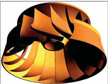
Figure 1.1: CFD-Based optimization result of a turbine runner.
(Wu et al., 2007)
1.1.2 Objective Functions
A target function is defined with a proper set of design parameters. To have a target function that properly integrates accurate physics models will yield results that comply with both geometric and dynamic parameters. The accuracy and relevance of the target functions of a CFD-based design loop is important since they must be evaluated several times until design specifications are met (Wu et al., 2007).
In order to establish the quality of the obtained shape after an optimization process, one must define an equation that include all criteria used as variables to improve such design. The optimum design will be the outcome of the minimization of this expression (Ferrano et al., 2004).
A possible definition of the objective function (OF) is an aggregation function with weighted coefficients ck - see Eq. 1.3-, defining the relevance factors of each single objective Fk with K
weighting coefficients ck, k=1,...,K , (Giannakoglou, 2002)
Faggr = K
X
k=1
ckFk(x) (1.3)
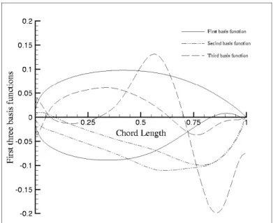
express the desired objective. One optimization approach defines the geometry of an airfoil as the linear combination of the optimization functions (in terms of aerodynamic parameters) and a set of perturbation functions, defined either analytically or numerically. These coefficients of the perturbation functions involved are then considered as the design variables. A set of such orthogonal basis functions - see figure 1.2 - are the functions to be evaluated to test a design alternative (Song and Keane, 2004).
Figure 1.2: Three numerically derived orthogonal basis functions. Source: Song and Keane (2004)
1.1.3 Optimization Methods
There are numerous methods available to do optimization over a given geometry, and multiple strategies can be applied to find the minimum of an objective function. The scope of the document is focused on commonly used methods for airfoil design. More optimization methods in airfoil design are reviewed in (Shyy et al., 2001; Vicini and Quagliarella, 1998).
An effective approach to wing airfoil design with optimal aerodynamic behavior is based on the solution of the inverse problems of aerodynamics. The desired characteristics of the wing airfoil are taken as input. An example can be a desired pressure map over the surface of the wing, the issue is to define the target pressure map since this pressure maps come usually from simulations or lab data. The output data is the shape that complies with the target coefficients. Other parameters like pressure distribution, drag coefficient, lift coefficient -to name a few- can be used as bounds for the wing airfoil (Abzalilov, 2005).
1.1.4 Heuristic Methods
lies in the time needed to find such solution, an exact method will need greater time to find a solution -if it indeed exist- than the heuristic approach. Then, when the type of problem and number of variables allows it, the applicability of heuristic methods on optimization problems is favored.
Other reasons that make heuristic methods attractive, or necessary, for complex problem solving are:
• Absence of a method to solve optimally the problem.
• Hardware limitations to apply exact method to solve the problem.
• Flexibility of the method that allow to incorporate difficult to model conditions.
• Use the method as part of a global procedure to obtain an optimum solution of the problem
To profit from an heuristic algorithm, certain properties should be considered:
• The computational cost is reasonable.
• The solution should be near optimal (with high probability).
• Obtaining a bad solution (far from optimal) should very unlikely.
There are many heuristic methods which difficult a full classification, and many of them are problem oriented, being used to solve an especific problem without possibility to generalize them to other uses (Marti and Gerhard, 2011).
An outline to place some known heuristics is (this is a wide take):
• Simulated annealing: With a hill-climbing approach for next solution finding, occasion-ally less optimum solutions are accepted. The idea is the probability of this happening decreases with time.
• Tabu search: It uses memory structures to avoid local optima. Tabu search inhibits the algorithm repeating previously made moves (To avoid the issue of simulated annealing).
• Swarm intelligence: This artificial intelligence technique is based on the idea of collective behavior. Two of the most known approaches are Ant Colony Optimization (ACO) and Particle Swarm Optimization (PSO). An advantage of swarm intelligence is that it is less prone to pursue local optima.
• Evolutionary Algorithms: A number of solutions (population) is considered simultane-ously, solutions are evaluated using ”survival of the fittest” criteria to find the optimum. this avoids the issue of premature convergence. This group is mentioned further.
• Support Vector Machines: They elaborate on Neural Networks. A convex objective function is used to overcome premature convergence.
Results can be directly obtained from heuristics or they can be combined with other optimiza-tion algorithms to improve their efficiency (e.g., obtain good seed values for gradient based techniques)
A commonly used approach for optimization processes is Evolutionary Algorithms. Specif-ically, the use of Genetic Algorithms (GAs), which are semi-stochastic semi-deterministic op-timization methods that are conveniently presented using the metaphor of natural evolution. The GAs are based on the evaluation of a set of solutions, called population. The population is treated with genetic operators: selection, crossover and mutation. All these operations include randomness. The main point is that the probability of survival of new individuals depends on their fitness: the best are kept with a high probability, the worst are rapidly discarded (Epstein and Peigin, 2006).
1.1.5 Gradient Based Techniques
Gradient based algorithms are the most used for local optimization. As their name states, they use gradient information to locate the optimum. Their use in engineering is widespread due to their efficiency (number of evaluations to find the optimum, possibility to include many design variables and the need for problem-specific tuning is low. The main drawbacks are: the ability to only find local optima, difficulty to solve discrete optimization problems, the algorithms are difficult to implement efficiently and are complex, they can be affected by numerical noise, this is covered in books such as (Haftka and G¨urdal, 1992).
Description
Gradient based methods make use of a two step process to find the optimum, it can be summa-rized as:
xq =xq−1+α∗Sq (1.4) The search direction S must be found first and then move in this direction until no more improvement is made, the second step is know as line search, which yields the optimum step sizeα∗. Nonetheless there are also gradient based methods that do not need a line search.
On most optimization problems, gradient information is obtained using finite difference cal-culations. This allows to estimate the gradient in a flexible way but becomes resource intensive and impact directly the optimization study. Also, the accuracy of finite difference depends on the step size chosen. If there is access directly to the source code, then an automatic differentiation can be implemented to obatin accurate gradient information.
The difference between algorithms rests in the criteria used to define the search direction. There are several algorithms used to find the best step size, combined with a gradient based algorithm to do the line-search. Some popular ones are: the golden section search, the Fibonacci search, and different variations of polynomial approximations.
If the gradient information is available, constrained local optimum can be corroborated with the Karush-Kuhn-Tucker (KKT) conditions which provide the requisites for a local optimum and read:
i. The optimum design point x* must be feasible.
ii. At such point the gradient of the Lagrangian vanishes
∇f(x∗) +
m
X
j=1
λj∇gj(x∗) + p
X
k=1
λm+k∇hk(x∗) = 0 (1.5)
where the lagrange multipliers λj ≥0 and λm+k are unrestricted in sign.
iii. For each inequality constraintλjgj(X) = 0, wherej = 1, m.
In unconstrained problems, the KKT conditions only need for the gradient of the objective function to vanish at X*. Also they are useful for identifying local optimum but cannot tell if a global optimum has been found.
Newton’s Method
The Newton algorithm is a classical gradient based optimization method, it is an unconstrained derived from a second order Taylor expansion of the objective function around an initial point x0
f(x)≈f(x0) +∇f(x0)T(x−x0) +1 2(x−x
0)TH(x0)(x−x0) (1.6)
H(x0) is the Hessian matrix with the second order gradient information of the objective function. Differentiating Eq. 1.6 respect to x and setting equal to zero in line with KKT conditions we obtain the update formula for the current design point:
x=x0−H(x0)−1∇f(x0) (1.7)
Unconstrained optimization
Two very popular methods are used for unconstrained problems, one is the Fletcher-Reeves and the other is the Broyden-Fletcher-Goldfarb-Shanno (BFGS). The Fletcher-Reeves(or conjugate gradient method) uses conjugate search directions to reach the optimum. This directions are created using information from the previous iteration. This method works well and will min-imize a quadratic function in theory in n or fewer iterations. it also requires small computer memory. The BFGS uses information from the previous n iterations to determine a new search direction. The method creates an approximation of the inverse of the Hessian matrixH(X0)−1 in Eq1.7. This approximation is updated after each iteration with new first order gradient in-formation. This method is superior to Fletcher-Reeves mathematically, but needs significatively more computer memory for the storage of the aprroximate inverse of the Hessian.
Constrained optimization
Constrained optimization problems can be adressed with Sequential Unconstrained Minimization Techniques (SUMT) (Fiacco and McCormick 68) and direct -or constrained- methods. The SUMT approach converts the problem to an equivalent unconstrained one in order to solve it (with any of the mentioned methods). This unsconstrained problem is obtained by penalizing the original objective function for constraint violations. The penalized objective function is obtained from:
fp(x, rp) =f(x) +rpp(x) (1.8)
Where f p(x) is the penalized objective function, rp is the penalization parameter and p(x)
the penalization function. A classical approach is to perform a minimization cycle forfp withrp
constant. When the unconstrained solution is achieved, rp is increased and the unconstrained
optimization cycle is done again. This gives a sequential movement towards the constrained optimum, the process is finished when convergence is achieved between succesive cycles. A popular example is the quadratic penalty function:
p(x) =
m
X
j=1
(max[0, gj(x)])2+ l
X
k=1
hk(x)2 (1.9)
The constrained optimum is approached from the infeasible region of the design space. There are also methods that approach from the feasible region. The value of the penalty parameter has a great influence on the performance of the algorithm, becoming a great drawback for these methods. Normally large values are used for satisfactory results, but this large values can lead to numerical ill-conditioning. This limitation may be overcome using the Augmented Lagrange multiplier method, it does so by using the Lagrangian to create a penalty function, and the estimate of the Lagrange multipliers to define penalty parameters. The advantage of this method is to give exact constraint satisfaction for a given value ofrp, being less sensitive to
SLP, takes the general non-linear constrained optimization problem and simplifies it to a linear equivalent by creating linear approximations of the objective and constraint functions around the current point. The optimum of these linear functions is found using an algorithm and then the resulting point is evaluated, a new set of linear approximations is created around this recently evaluated point. The main drawback is the sensitivity to move limits and it might not always yield a feasible solution, hence MMFD or SQP are preferred.
MMFD is based on the feasible directions method. A modification was introduced to this method to yield a search direction which follows the active constraint bounds towards the opti-mum. This algorithm is widely used on structural optimization due to its robustness and ability to find the feasible design space rapidly.
SQP is very popular for engineering optimization applications. A quadratic approximation of the objective function and linear approximations of the constraint functions are used to find a search direction. Usually a penalty function is used to define the step size in this direction. A new design point is then obtained from combination of the search direction and optimum step size (from Eq. 1.4), this new design point is then evaluated and the process iterates until convergence (Blockley and Shyy, 2010).
Steepest Descent
The steepest descent method is an iterative procedure used to accomplish optimization. Starting from some initial geometry the best direction to move towards is the direction of the steepest descent. This direction corresponds to the negative of the gradient. That is:
sn+1 =sn−β ∇(f(s
n))
k ∇(f(sn))k (1.10)
whereβ is a constant to be determined (in an optimum way) and the gradient atsn off(s) can be approximated by forward-difference:
∂f(s) ∂si sn
= f(s
n+4s
i)−f(sn)
4si
(1.11)
or with a second order central-difference approximation (Haftka and G¨urdal, 1992):
∂f(s) ∂si sn
= f(s
n+4s
i)−f(sn− 4si)
24si
(1.12)
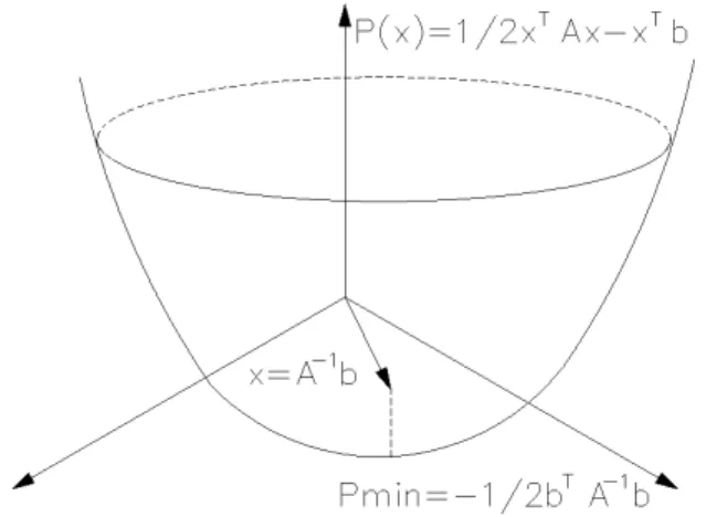
Figure 1.3: Steepest descent on a given space (local-global minima) Source: Garcia (2007)
1.2
Aerodynamic Forces and Moments
Aerodynamic forces are the reactions of a body moving through a fluid. Pressure and shear stress distributions on the body surface are the acting forces that make flight possible. Different force scenarios can be observed depending on the orientation of the body. Pressure (p) acts in the normal direction to the body and shear (τ) acts tangentially (see figure 1.4). The effect of p and τ distributions integrated over the complete body surface is a resultant aerodynamic forceR and momentM on the body. R can be split into two components lift (L) and drag (D) (Anderson, 2001).
1.3
Optimization In Computational Fluid Dynamics
CFD has come a long way since its beginnings. The speed and capacity of the hardware to ma-nipulate huge sets of data has increased considerably. This capacity allows to simulate complex fluid flow situations. Problems that were previously addressed with different disciplines are now approachable taking advantage of CFD. The robustness offered by current CFD codes to solve the governing flow equations, enable designers to obtain accurate preliminary field data to esti-mate the response of new objects from virtual prototypes. One of the advantages of using CFD analysis for optimization is to have multiple sets of data available at the same time (volumetric fields). The possibility to analyze transient flow cases gives a head start to understand the behavior of object in more realistic scenarios. Multiple efforts have been carried out regarding coupling of CFD analysis and design optimization, several in-house codes have been developed as well as existing cad tools and code integration.
As technological improvement and competition require more careful optimization of designs or, when new high-technology applications demand prediction of flows for which the database is insufficient, experimental development may be too costly and/or timeconsuming. Optimization in these areas can produce large savings in equipment and energy costs and in reduction of environmental pollution (Ferziger and Peric, 2002).
The calculations obtained from CFD can be used for optimization regardless of the complete accuracy of the model. The predictions obtained when turbulence models are used are not accurate enough that they can be accepted quantitatively without testing. However, the trends may be accurately reproduced so that the design predicted to be the best by the model also performs the best in tests. Calculations based on turbulence models can reduce the number of experimental tests required and thus reduce the cost and the time required for development of a new product (Ferziger and Peric, 2002).
The use of k-epsilon turbulence model is quite popular, although it has been known that there is a deficiency in its performance for problems involving rotation and curvature, the standard k-epsilon turbulence model is widely used in studies for the steady-state turbulent flow calculations, due to its robustness in practical applications (Wu et al., 2007).
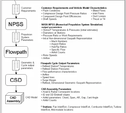
Multidisciplinary Optimization (MDO) presents optimization on a new perspective. MDO integrates CAD softwares to control design parameters and CFD simulation softwares to acquire the data to evaluate objective functions (Dye et al., 2007). Optimization then has a physics based data to evaluate design options. The modeling of gas turbines are among the most complex systems available, a cad based parametric approach has rendered interesting results using the following methodology (see Fig.1.5 ).
Figure 1.5: Engine Cycle Modeling System Components and Input/Outputs Source: Dye et al. (2007).
containing discontinuities. In Navier-Stokes computations, the scheme is usually applied to the approximation of convective terms (Epstein and Peigin, 2006).
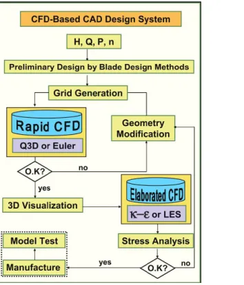
A computational fluid dynamics-based design system with the integration of three blade de-sign approaches, automatic mesh generator and CFD codes enables a quick and efficient dede-sign optimization of turbine components. This examples include sophisticated Large Eddy Simula-tions (LES) in a Francis turbine and in a centrifugal pump impeller at design and off-design conditions. However, a robust and fully 3D inverse design approach, by which the required flow characteristics and parameters are specified as inputs and the corresponding blade geometry is computed and generated as output, is still not commonly implemented. The governing equa-tions for this phenomena are for turbulent flow, but the current assumpequa-tions still dwell on the inviscid approach. A viscous CFD solver is needed. The design has to be evaluated by the solver and the solution must be updated to modify the input (Wu et al., 2007). The inviscid Quasi 3-Dimensional (Q3D) codes by means of both finite difference method and FEM incorporated into this system are primarily employed in the preliminary optimization stages due to their rapid convergence rate and reliability. Using the methodology described in Fig.1.6 a francis turbine is optimized. Developed for nearly 2 decades, mesh handling and generation, CFD analysis and design optimization is integrated under one single iterative process. As an example, on the right hand side of the figure, a redesigning the vanes of the runner is shown.
Figure 1.6: Left: CFD-Based Design System. Right: Optimized guide vane and stay vane profiles
Source: Wu et al. (2007).
prediction and massive multilevel parallelization of the whole computational framework. This methods highlights are multipoint wing optimization for transport type aircraft configurations (see Fig. 1.7).
Figure 1.7: Original(Left) and Optimized (Right) ARA M-100 wing-body configuration. Pres-sure distribution on the upper surface of the wing at M = 0.80,CL = 0.50.
Reducing in the drag even in 1% would yield noticeable results in th pay-load of the aircraft (Epstein and Peigin, 2007). It was proven that this method allows to design feasible aerodynamic shapes which:
• Possess a low drag at cruise conditions;
• Satisfy a large number of geometrical and aerodynamic constraints (15-20 per design);
• Offer a good off-design performance in markedly different flight conditions such as take-off and high Mach zone.
1.4
Shape derivative
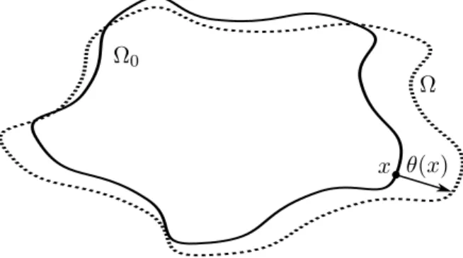
A more recent approach in shape optimization computes the derivative of the objective function with respect to the domain. It is a formal method and it has been shown to have excellentes results in solid mechanics problems. Applications of direct shape derivatives to fluids has been explore by Mohammadi and Pironneau (2010) and others. The main idea is to evolve the domain boundary according to a sensitivity analysis. Although the domain deformation can require remeshing and topology changes can cause problems on the boundary evolution, the explicit definition of the domain boundary is a great advantage. The optimization process is based on the variation of the domain boundaries that evolve to an optimum shape (Allaire, 2006; Dapogny, 2013). These method is based on the Hadamard shape derivative Hadamard (1909). A variation on the domain shape (without changing the topology) can be defined with a displacement field θ and the initial domain Ω0 (See Fig. 1.8). Assuming θ sufficiently small,
a deformed domain Ω is represented by Ω = (I +θ)(Ω0). The shape variations (I +θ) are
considered homeomorphisms close to the identity.
θ(x) Ω0
Ω
x
Figure 1.8: Hadamard’s shape variation
Shape optimization method based on Hadamard boundary variation using differentiation with respect to the domain was implemented by Betancur et al. (2014) and compared to a topology optimization using a homogenization method based on the Brinkmann penalization.
Automatic CFD Coupled Optimization
2.1
Description
The main objective is to produce a method that optimizes the shape of an aerodynamic profile. To achieve this, we must define first the set of needs towards the construction of the method itself. The process begins with the identification of the disciplines to integrate:
i. Shape parametrization.
ii. Geometry manipulation.
iii. Aerodynamics.
iv. CFD-Based shape optimization.
v. Optimization methods (Gradient-based).
The steps to follow become the sewing thread among the disciplines mentioned above. They conform a road map of the whole process. The following list describes the initial necessary definitions:
• The geometry is defined as the input and target of the method.
• A set of design variables are defined (they are a requirement of the method).
• The optimization function is defined according to some criteria.
From which a set of needs are identified to comply with the previous steps and the optimization process. The needs are listed below:
• The geometry has to be represented as a data set that is portable between the multiple tools.
• The geometry has to be prepared for CFD analysis, including generation of the domain and boundary conditions.
• A CFD solver must be chosen to fulfill fluid analysis requirements.
• The selected CFD solver must be adapted to allow evaluation of the optimization function.
• The optimization function must be evaluated and updated during run time.
• The geometry has to be manipulated based on the optimization method and criteria.
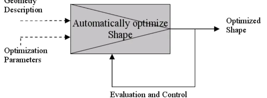
2.1.1 Main Function and Flows Abstraction (Black Box)
If the process is contemplated as a black box it can be simplified to basic input/output (I/O) variables. The main I/O variables will begin the definition of the structure of the method. During any design process, feedback is an important step before any design alternative is chosen. The expertise of the designer can accelerate an optimization process avoiding stagnation in local minima. This reason supports the need to offer a degree of interaction between the optimization process and the user. The combination of an experienced designer, a solid design process and effective tools guarantee the achievement of an optimal solution.
Finding optimal solutions with the minimal effort is foremost the objective to achieve, and reducing the problems to its general form help to address their solution. Basically, the process can be reduced to the following need:
• An application that integrates a set of tools to test and analyze automatically an aerody-namic profile.
Then a black box representation like in Fig. 2.1states the design process.
Figure 2.1: Black Box Representation of the Method
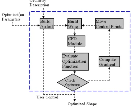
2.1.2 Functional Synthesis
solution methods). Specific solutions to each particular need are only selected after a generalized segregation process. This strategy also reveals the subdivision of functions and the expected interaction between them, then data structures can be considered. The data structure must obey to the set of needs and how they develop throughout the problem, not the other way around.
Figure 2.2: Function decomposition
In Fig 2.2an overall decomposition in basic sub-modules can be appreciated. The process can be subdivided into functions which form the underlying structure of the optimization. Both geometric and optimization parameters must be set in the early stage. The first module takes care of the initial geometric representation and conservation of the parameters. A following module expands the geometry to a 3d body from parameters specified earlier. Then, one module groups CFD pre-processing, solving and post-processing using the geometry provided by the previous module. The post-processed data is fed to a module that evaluates the optimization function. At this point a check point is set to identify wether the optimum has been reached. The gradient is calculated in another module in order to set the direction for the geometric change. In a subsequent module, the gradient is used to modify the shape by moving the control points. At last this modified shape is the input for another optimization cycle. When the module structure is considered the tools that must be developed to solve each portion of the problem arise clearly.
to displace the control points in the opposite gradient direction is noticed also in the rate of convergence and speed of the method. Variables such as meshing parameters, discretize the CFD domain in smaller elements (therefore increasing the number of them) increasing the time consumed by each simulation to complete.
2.2
Shape Optimization Tests and Results
The algorithm was tested using 6 different geometries, 3 of them were NACA profiles. The results observed in the NACA standard profiles reduce the drag coefficient, even though these profiles have been thoroughly tested already. The other 3 geometries are the proof of concept examples, they help to expand the understanding of the job done by the algorithm.
Altough the outlines of the process done by the algorithm have been described, a more detailed and computational oriented descripition is given:
i. The proper variables are instantiated in memory.
ii. The parameters file is read (defined in the file parameters.txt insisde the case folder), it contains data such as:
(a) Number of control points.
(b) The number of segments (nn) to generate between the control points when converting to polyline.
(c) The control points themselves (X andY coordinates).
(d) Triangle 2D meshing Parameters (maximum triangle area and triangle switches).
(e) Netgen Volume meshing parameters ( element size and mesh fineness).
(f) Optimization parameters (delta to move points and weight factor for the gradient)
(g) Foil parameters (Wing lenght, attack angle and tapper angle).
(h) Status flag (to stop the application during run time).
iii. The curve that describes the airfoil is generated from the control points.
iv. The curve is converted into a polyline
v. The polyline is passed to triangle and the airfoil is triangulated.
vi. The triangulated airfoil is converted to a 3D wing (The wing can be optionally written to an STL file).
vii. The wing is used to construct the CFD domain in netgen format.
viii. The OpenFOAM case is created (using the dummy case with inlet velocity, kinematic viscosity and turbulence parameters)
ix. The CFD domain is converted to OpenFOAM format and written in the case folder.
xi. The solved case is post processed and initial Drag and Lift coefficents are obtained.
xii. A control point is displaced.
xiii. The polyline is reconstructed from the modified curve.
xiv. The meshing process takes place again.
xv. The CFD domain is reconstructed.
xvi. A new case for the new geometry is created.
xvii. The new case is solved and new Drag and Lift coefficients are calculated.
xviii. The objective function is evaluated.
xix. The gradient is calcualted and stored.
xx. The steps between xii andxix are repeated until all the control points have been moved.
xxi. The geometry is modifed using the direction of the gradient and the weighing factor.
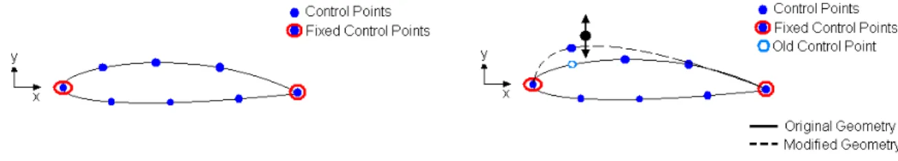
(a) Airfoil defined by its control points (b) Displacement of a control point
Figure 2.3: Control point description and modification of an airfoil
It is to be expected from aerodynamic principles that a decrease in drag will carry on a decrease in lift. The objective is to achieve a decrease of drag with the minimal lift loss possible. This initial tests are presented to demonstrate the concept, far from offering a solution to the requirements of the industry.
In Fig. 2.3 the basic concept of the control points that describe the airfoil curve is displayed. Two control points remain fixed (the ones that define the chord length), the rest are the ones to be displaced. Each control point can be moved in the Y direction by a quantity defined in the parameters file. Each displacement of a control point brings forth a new shape to be evaluated.
2.2.1 Conceptual Examples
Airfoil raw Example
in the upper surface and 2 control points on the lower surface (given that the extremes remain fixed) a pronounced change in shape was observed. The settings for this example can be observed in table2.1.
Table 2.1: Airfoil raw example initial conditions and settings
Variable Value
Inlet velocity 50m/s (or 180 km/h) Kinematic viscosity 1e-05 m2/s
Number of control points 5 CFD domain number of elements 2316
Attack angle 0◦
In figure2.5 the change in shape can be observed. Other changes that can be observed are: the change of the pressure map over the surface of the wing, a drop in the drag coefficient and also a consequent drop in lift coefficient.
(a) initial surface mesh for airfoil raw (b) final surface mesh for airfoil raw
Figure 2.4: Airfoil raw example surface mesh transformation
Airfoil Example
The second example is similar to the airfoil raw, the difference is the number of control points and how the coefficients for the optimization function were used. With higher number of control points a higher degree curve can be defined. More control points increase the size of the search space because each control point translates into a CFD scenario. The settings for this case are displayed in table 2.2.
In Fig. 2.6the change of shape in the direction of the gradient can be observed. The change is greater in the front which induces most of the drag. In the rear a combed shape emerges on the lower surface, which is commonly observed in airfoils to induce lift.
(a) initial u and p fields for airfoil raw (b) final u and p fields for airfoil raw
Figure 2.5: CFD visualization of the airfoil raw case
Table 2.2: Airfoil example initial conditions and settings
Variable Value
Inlet velocity 50m/s (or 180 km/h) Kinematic viscosity 1e-05 m2/s
Number of control points 12 CFD domain number of elements 6315
Attack angle 0◦
(a) initial surface mesh for airfoil (b) final surface mesh for airfoil
Figure 2.6: Airfoil example surface mesh transformation
Cylinder Example
(a) initial u and p fields for airfoil (b) final u and p fields for airfoil
Figure 2.7: CFD visualization of the airfoil case
were needed. Having more control points ensure smoothness of the shape. The settings for this case are displayed in table 2.3.
Table 2.3: Cylinder example initial conditions and settings
Variable Value
Inlet velocity 66.81 m/s (or 240 km/h) Kinematic viscosity 1e-05 m2/s
Number of control points 18 CFD domain number of elements 3086
Attack angle 0◦
In Fig. 2.8 the change of shape in the direction of the gradient can be observed. The change is appreciated as the geometry is stretched to make it more streamlined. The area reduced in height is increased in width, but the change is slight.
(a) initial surface mesh for cylinder (b) final surface mesh for cylinder
In Fig. 2.9the change of shape induced a reduction of the pressure experienced by the geometry when in contact with the flow. Also a more flattened geometry reduced the speeds of the fluid surrounding.
(a) initial u and p fields for cylinder (b) final u and p fields for cylinder
Figure 2.9: CFD visualization of the cylinder case
2.2.2 Optimization of NACA airfoils
In the set of NACA airfoils, the contour was obtained from (Trapp and Zores, 2007). This Java applet generates the x and y coordinates for many 4 digit NACA foils. The minimum number of control points available to describe the airfoil were used (10 for each upper and lower curve). Having a reduced set of control points reduces the search space, then the whole run for the application takes less time. Remember that for each control point perturbed a complete CFD simulation case is generated (see Fig. 2.10).
The set of NACA foils were not altered as much as the other examples, but the slightest variation to this standard and tested profiles proved to change their coefficients considerably. In Fig. 2.11the change in shape may not be noticeable, but when the results from the coefficients are read, the difference can be seen. A considerable change is also noticeable in the pressure distribution see Fig. 2.12 and notice the data bars. This type of visualization can be obtained when using full CFD approaches. Each CFD simulation holds field data useful for multiple analysis beyond the objective functions only. A change is observed in the performance of the wing rather than in the mesh shape.
NACA0030 Example
The settings for this case are displayed in table2.4.
NACA0022 Example
Figure 2.10: Case structure of an optimization
Table 2.4: NACA0030 example initial conditions and settings
Variable Value
Inlet velocity 50 m/s (or 240 km/h) Kinematic viscosity 1e-05 m2/s
Number of control points 18 CFD domain number of elements 9854
Attack angle 0◦
Table 2.5: NACA0022 example initial conditions and settings
Variable Value
Inlet velocity 50 m/s (or 240 km/h) Kinematic viscosity 1e-05 m2/s
Number of control points 18 CFD domain number of elements 14089
Attack angle 0◦
NACA0012 Example
(a) initial surface mesh for NACA0030 (b) final surface mesh for NACA0030
Figure 2.11: NACA0030 example surface mesh transformation
(a) initial u and p fields for NACA0030 (b) final u and p fields for NACA0030
Figure 2.12: CFD visualization of the NACA0030 case
Table 2.6: NACA0012 example initial conditions and settings
Variable Value
Inlet velocity 2.78 m/s (or 240 km/h) Kinematic viscosity 1e-05 m2/s
Number of control points 18 CFD domain number of elements 7326
Attack angle 0◦
2.2.3 Overall review of results
(a) initial u and p fields for NACA0022 (b) final u and p fields for NACA0022
Figure 2.13: CFD visualization of the NACA0022 case
(a) initial u and p fields for NACA0012 (b) final u and p fields for NACA0012
Figure 2.14: CFD visualization of the NACA0012 case
Table 2.7: Comparison between coefficients
Example Name Cd Cd new % diff Cl Cl new % diff
Conclusions and Future Work
3.1
Conclusions
A method for the CFD analysis and simulation of aerodynamic profiles is presented on this work. The proven concept was to develop an infrastructure for shape optimization of an aerodynamic profile using a gradient-based method. This is an example of the kind of work that only can be achieved in a virtual Wind Tunnel. After intensively selecting the optimization criteria and constants a satisfactory condition was achieved. When pursuing an objective like reducing drag, lift is proportionally reduced as well since they are directlly related.
An optimal combination of forces is the objective of the method. An accurate definition of the constants that define the weight of the objectives becomes a crucial step. When only a minimization of drag is treated, the geometry differs greatly from the initial, but the significant loss of lift leads to profiles with no capacity to sustain flight conditions optimally. For this matter, a penalization of lift and minimal area acceptable were introduced.
The possibility of exploring drag minimization exclusively in aerodynamic design poses in-teresting results. Using the developed method with switches for specific design scenarios (auto-motive, hydrodynamic) offers feasible and improved shapes.
One of the main concerns during the tests was the quality of the mesh. The high curvature involved in the leading edges of airfoils forced the need for increased number of surface elements, this translated into elevated number of tetrahedra in the CFD domain volumetric mesh, inducing high demands on computational operations and amounts of disk space.
Coarser meshes allow the designer to have valuable initial approximations. If an accurate mesh grade is defined, even if coarse, the designer can obtain shape optimization within minutes. The ability of the code to define a shape with few control points presents an important advantage when the optimization process occurs. The dimension of the search plays a vital role when defining the evolution of the shape, having fewer control points reduces the size of the search space, enabling the designer to obtain initial approximations faster.
high Reynolds numbers lead to the assumption of a steady state flow condition, the k-epsilon model is used widely.
The process of constructing the shape in 3d from 2d control points and later on the CFD domain became a time consuming task. A parametrical definition of the geometry was imple-mented and allows the generation of various shapes with a valid CFD domain. The CFD domain size is quite large when treating outside flows (like the ones when simulating an airfoil moving through air) and causes simulation times to increase considerably.
3.2
Future Work
After proving the concept of CFD-based shape optimization in a single CPU, the code will undergo changes to allow parallelization. Parallelization will allow more complex geometries, more refined domains and shorter simulation times.
The current meshing process has to be reviewed for efficient adaptation to CFD optimal conditions, possible use of more specific airfoil hexahedra mesh generation will be explored using OpenFOAM’s embedded mesher “blockMesh”.
D. F. Abzalilov. Minimization of the wing airfoil drag coefficient using the optimal control method. Fluid Dynamics, 40(6):985–991, 2005.
@Aerospaceweb. Lift and drag vs. axial force. Web, 2007. Available at: http://www. aerospaceweb.org/question/aerodynamics/q0194.shtml.
G. Allaire. Conception optimale de structures: Majeure Sciences de l’ing´enieur, simulation et mod´elisation. ´Ecole polytechnique, D´epartement de Math´ematiques appliqu´ees, 2006. ISBN 9782730213042.
John D. Anderson. Fundamentals Of Aerodynamics. Mc Graw-Hill, 3rd edition, 2001.
Esteban Betancur, Pascal Frey, Charles Dapogny, and Manuel J. Garc´ıa. A two step cfd op-timization process: Topology and shape opop-timization. In 11th World Congress on Com-putational Mechanics (WCCM XI) 5th European Conference on ComCom-putational Mechanics (ECCM V) 6th European Conference on Computational Fluid Dynamics (ECFD VI), page 2, July 2014.
R. Blockley and W. Shyy. Encyclopedia of Aerospace Engineering. John Wiley & Sons, Ltd., 2010.
Charles Dapogny. Shape optimization, level set methods on unstructured meshes and mesh evolution. PhD thesis, Ecole Doctorale Paris Centre, 2013.
Christopher Dye, Joseph B. Staubach, Diane Emmerson, and C. Greg Jensen. Cad-based para-metric cross-section for gas turbine engine mdo applications. Computer Aided Design and Applications, 4(1-4):509–518, 2007.
B. Epstein and S. Peigin. Optimization of 3d wings based on navier-stokes solutions and genetic algorithms. International journal of Computational Fluid Dynamics, 20(2):75–92, 2006.
B. Epstein and S. Peigin. Accurate cfd driven optimization of lifting surfaces for wing-body configuration. Computers and Fluids, 2007.
Lluis Ferrano, Jean-Louis Kueny, Francois Avellan, and Laurant Pedretti, Camille Tomas. Sur-face parameterization of a francis runner turbine for optimum design. 22nd IAHR Symposium on Hydraulic Machinery and Systems, 2004.
Manuel Garcia. Fixed Grid Finite Element Analysis in Structural Design and Optimisation. PhD thesis, Department of Aeronautical Engineering, The University of Sydney, March 1999.
Manuel J. Garcia. Lecture notes on numerical analysis, 2007.
K. C. Giannakoglou. Design of optimal aerodynamic shapes using stochastic optimization meth-ods and computational intelligence. Progress in Aerospace Sciences, 38:43–76, 2002.
Jacques Hadamard. M´emoire sur le probl`eme d’analyse relatif `a l’´equilibre des plaques ´elastiques encastr´ees. Paris : Imprimerie nationale., paris : imprimerie nationale. edition, 1909.
R. Haftka and Z. G¨urdal. Elements of Structural Optimization. Kluwer Academic Publishers, 3rd edition, 1992.
Rafael Marti and Reinelt Gerhard.The Linear Ordering Problem - Exact and Heuristic Methods in Combinatorial Optimization. Springer, 2011. Chapter 2, Heuristic Methods.
Bijan Mohammadi and Olivier Pironneau. Applied Shape Optimization for Fluids. Oxford University Press Inc., 2010.
R. T. Rockafellar. Fundamentals of optimization, 2007.
Ruber A. Ruiz and Manuel J. Garc´ıa. Shape optimization of a gas injector. In 11th World Congress on Structural and Multidisciplinary Optimization, Sydney, Australia, June 2015. URLhttp://www.issmo.net/wcsmo11/papers/1352_paper.pdf.
Wei Shyy, Nilay Papila, Rajkumar Vaidyanathan, and Kevin Tucker. Global design optimization for aerodynamics and rocket propulsion components. Progress in Aerospace Sciences, 37:59– 118, 2001.
Wenbin Song and Andrew J. Keane. A study of shape parameterisation methods for airfoil optimisation. AIAA, page 1, 2004.
Jens Trapp and Robert Zores. Applet to generate naca 4 digit airfoils. Web, November 2007.
http://www.pagendarm.de/trapp/programming/java/profiles/NACA4.html.
A. Vicini and D. Quagliarella. Airfoil and wing design through hybrid optimization strategies. AIAA, pages 27–29, 1998.