Optimal Workers Allocation for the Crossdocking Just in Time Scheduling Problem

Texto completo

(1)INSTITUTO TECNOLÓGICO Y DE ESTUDIOS SUPERIORES DE MONTERREY CAMPUS MONTERREY DIVISIÓN DE INGENIERÍA Y ARQUITECTURA PROGRAMA DE GRADUADOS EN CIENCIAS DE LA INGENIERÍA. OPTIMAL WORKERS ALLOCATION FOR THE CROSSDOCKING - JUST IN TIME SCHEDULING PROBLEM. THESIS PRESENTED AS A REQUIREMENT TO OBTAIN THE DEGREE OF:. DOCTOR OF PHILOSOPHY IN ENGINEERING MAJOR IN INDUSTRIAL ENGINEERING. GUILLERMO ARTURO ÁLVAREZ PÉREZ. MAY OF 2007.

(2) INSTITUTO TECNOLÓGICO Y DE ESTUDIOS SUPERIORES DE MONTERREY CAMPUS MONTERREY DIVISIÓN DE INGENIERÍA Y ARQUITECTURA PROGRAMA DE GRADUADOS EN CIENCIAS DE LA INGENIERÍA. The members of this committee recommend that the thesis of Guillermo Arturo Álvarez Pérez be accepted as a partial requirement to obtain the degree of: Doctor of Philosophy in Engineering Major in Industrial Engineering. Thesis committee:. ____________________________ José Luis González Velarde, Ph. D. Advisor. ______________________ John Welsh Fowler, Ph. D. Co-advisor. _______________________ Jorge Limón Robles, Ph. D. Synodal. _____________________________ Neale Ricardo Smith Cornejo, Ph. D. Synodal. ____________________________________ Francisco Román Ángel Bello Acosta, Ph. D. Synodal. APPROVED. ___________________________________ Francisco Román Ángel Bello Acosta, Ph. D. Director of the Graduate Program in Sciences of Engineering.

(3) Dedicatory. To God. To my wife Azalea. To my daughter Andrea. To my parents Alfonso and Consuelo. To my siblings Alfonso, Érika and Diana. To all the people I love. To the President of México, Felipe de Jesús Calderón Hinojosa.

(4) Acknowledgements. I am deeply grateful to my thesis advisor, Dr. José Luis González Velarde, for his help and guidance during all these years. I am also grateful to the members of my thesis committee, Dr. John Welsh Fowler, Dr. Jorge Limón Robles, Dr. Neale Ricardo Smith Cornejo, and Dr. Francisco Román Ángel Bello Acosta, for their comments and suggestions. I thank all of the faculty members and classmates that are part of the Doctoral Program in Industrial Engineering at Tecnológico de Monterrey. Finally, I want to acknowledge the financial support received from Tecnológico de Monterrey through grant number CAT025 to carry out this work..

(5) Abstract. In this work, a warehouse is allowed to function as a crossdock to minimize costs for a scheduling problem. These costs are due to two factors: the number of teams of workers hired to do the job, and the transit storage time for cargo. Each team of workers has a fixed cost per working day, and the cargo can incur early and tardy delivery costs. Then, the transit storage time for cargo is minimized according to Just in Time (JIT) scheduling. The goal is to obtain both: the optimal number of teams of workers in the crossdock and a schedule that minimizes the transit storage time for cargo. An integrated model to obtain both the optimal number of teams of workers and the schedule for the problem is written. The model uses the machine scheduling notation to describe it. Since the problem is known as NP-hard, a solution approach based on a combination of two metaheuristics, Reactive GRASP embedded in a Local Search algorithm and Tabu Search (RGLSTS), is provided. The results obtained from the exact method that uses the ILOG CPLEX 9.1 solver for 14 problem instances and the results obtained from the RGLSTS metaheuristic algorithm for the same problem instances are discussed. This research has an important academic contribution because it involves the development of a metaheuristic algorithm not previously applied to a relevant problem that has not received attention. Besides, the source codes of the programs that solve the problem are available for the reader and they can be modified according to the user needs. In the industry field, the algorithm mentioned above can be easily adapted in order to be applied to a real problem (i.e., large transshipments in companies like Wal-Mart, HEB, among others). Obtaining optimal or near optimal solutions for the problem of this work represents an improvement in the movement or distribution of the workforce and products, reducing this way, hiring costs, transportation costs and inventory costs.. i.

(6) Key words: Workers allocation, Just in Time scheduling, machine scheduling, crossdocking, metaheuristics.. ii.

(7) Contents. Chapter 1. Introduction................................................................................................. ............ ...... 1. 1.1 Thesis. ............. Structure……..……………………….………….………...….....…....... 4. 1.2. ............. Methodology................................................................................................ 4 Chapter 2. Chapter 3. Problem. ............. Description........................................................................................ 6. 2.1 Literature. ............. Review.......................................................................................... 8. 2.2 Relationship of the Problem with Machine. ........... Scheduling…............................. 12. 2.3 Model for the. ........... Problem.……………………………………..………………....... 17. Heuristics and. ........... Metaheuristics......................................................................... 26. 3.1. ........... Heuristics……………………........................................................................ 26 3.2. ........... Metaheuristics………………….................................................................... 27 3.2.1. .......... GRASP…………………………………………………………………. 29 ... 3.2.2 Tabu. ........... Search…………………………………………………………...... Chapter 4. 31. Solution Approach for the Crossdocking - Just in Time Scheduling Problem........................................................................................................ .......... ..... 35. 4.1 Solution. ........... Form…………................................................................................. 35. iii.

(8) 4.2 Exact Method of. ........... Solution…………............................................................... 36. 4.3 Alternative Method of. ........... Solution…………....................................................... 38. 4.3.1 Solutions. ........... Construction………………………………………………..... 4.3.2 Solutions. ........... Improvement………………………………………………….. ........... Experiments......................................................................... 51. Results………….................................... Chapter 6. Appendixes. 46. 4.4 Computational. 4.4.1 Testing and Comparison of. Chapter 5. 38. .......... 52. Solution Approach for the Optimal Workers Allocation for the Crossdocking - Just in Time Scheduling. ........... Problem....................................... 56. 5.1 Exact Method of. ........... Solution…………............................................................... 56. 5.2 Alternative Method of. ........... Solution...................................................................... 58. 5.3 Model for the Problem (reduced. ........... version)……………………………………... 61. Conclusions........................................................................................................... ..... 69. 6.1 Future. ........... Work…………................................................................................... 70. ...................................................................................................................... .......... ...... 72. Appendix 1 Linear and Integer. ........... Programming..................................................... 72. Appendix 2 Integer Programming Model for the Crossdocking - JIT Scheduling Problem Instance shown in Table. ........... 4.1.......................... 76. Appendix 4 Output of the RG Algorithm for a Crossdocking - JIT Scheduling Problem. ........... Instance............................................................................ 79. Appendix 5 Output of the RGTS Algorithm for the Crossdocking - JIT Scheduling Problem Instance shown in Appendix. iv. ...........

(9) 4....................... 82. Appendix 9 Results of the RG and RGTS Algorithms for the 16 Crossdocking - JIT Scheduling Problem Instances shown in. ........... Appendix 8............. 84. Appendix 11 Results of the RGLS and RGLSTS Algorithms for the first 14 Optimal Workers Allocation for the Crossdocking - JIT Scheduling Problem Instances shown in Appendix. ........ 103. 8.................... References. ...................................................................................................................... ........ 122 ...... Vita. ...................................................................................................................... ........ 127 ...... v.

(10) List of Figures 1.1. a) Earliness function; b) Tardiness function; c) Earliness-tardiness function. These three functions have a common due date d. 2.1. A crossdock flow. 2.2. a) A representation of the sources or predecessors of an outgoing container j; b) An example of an Sij matrix with 4 incoming containers and 2 outgoing containers. 2.3. A more detailed flow for the crossdocking - JIT scheduling problem. 2.4. Inbound or outbound area of the crossdocking - JIT scheduling problem seen as an assignment - scheduling problem. 3.1. Pseudo-code for a basic GRASP procedure. 3.2. Pseudo-code for a basic Tabu Search procedure. 4.1. Solution for a crossdocking - JIT scheduling problem instance: a) Assignment; b) Scheduling. 4.2. Pseudo-code for the RG algorithm. 4.3. An example of the ejection chain process: a) Before the movement of the job[j]; b) After the movement of the job[j]. 4.4. Graphical sequence of the output of an iteration of the RG algorithm for the inbound area of the crossdock. 4.5. Movements. of. the. algorithm:. InsertRightSameMachine(πk(i));. a). InsertLeftSameMachine(πk(i));. InsertDifferentMachine(πk(i),. c). πq);. b) d). ExchangeSameMachine(πk(i)); e) ExchangeDifferentMachine(πk(i), πq(j)) 4.6. Pseudo-code for the TS algorithm. 4.7. RGTS solution: a) Tabular form; b) Machine-Job form; c) Graphical form (only inbound area). 4.8. Input file structure for the exact model algorithm and for the RGTS algorithm. 5.1. Pseudo-code for the RGLS algorithm. 5.2. Assignment of the initial values for the number of breakdown and buildup machines for the RGLS algorithm. 5.3. Neighborhood of the point (m, M). This point represents the current number of machines rented in the inbound and outbound areas of the crossdock, respectively. vi.

(11) List of Tables. 2.1. Percentage of occupation of the technological coefficients matrix for different crossdocking JIT scheduling problem instances. 4.1. Input data for a crossdocking - JIT scheduling problem instance with 4 incoming jobs and 2 breakdown machines, and 3 outgoing jobs and 2 buildup machines. 4.2. Input parameters {ri, pi, di} for a crossdocking - JIT scheduling problem instance with 10 incoming jobs and 2 breakdown machines. 4.3. Input data for a crossdocking - JIT scheduling problem instance with 10 incoming jobs and 2 breakdown machines, and 11 outgoing jobs and 3 buildup machines. 4.4. Experimental results of our solution approach for the crossdocking - JIT scheduling problem. 4.5. Comparison of results of our solution approach with other authors’ solution approach for the crossdocking - JIT scheduling problem. 4.6. Average objective values for the RG algorithm when using the 4 different greedy functions separately. 5.1. Experimental results for the complete version of the optimal workers allocation for the crossdocking - JIT scheduling problem when using the integer programming solver ILOG CPLEX 9.1 with default parameters. 5.2. Experimental results of the optimal workers allocation for the crossdocking - JIT scheduling problem when using the RGLSTS algorithm. 5.3. Experimental results for the reduced version of the optimal workers allocation for the crossdocking - JIT scheduling problem when using the integer programming solver ILOG CPLEX 9.1 with specific parameters. vii.

(12) Chapter 1. Introduction. Logistics, and particularly, inventory, transportation, scheduling, and workforce allocation are important activities within factories and they play a central role in the operations research field. Their study has led to the development of many models and algorithms which have also been applied to other scientific, academic, and industrial fields. These topics are complex and they involve many variables, uncertainties, and costs. Most of the time, the objective is to optimize results, i.e. to maximize profits or minimize costs, taking into consideration the available resources assigned to it. Very often, to do this, it is necessary to use sophisticated models and optimization techniques as well as powerful information technology [Crainic and Laporte (1998)]. The scheduling activity is strongly related to manufacturing, inventory, and transportation. Scheduling can help the manufacturing industry to reduce production and inventory costs. Also, it can help the transportation industry to reduce transportation costs. Obtaining optimal or near optimal solutions to problems related to these areas represents an improvement in the production as well as in the movement or distribution of the products. This is one of the reasons why the scheduling area is so important nowadays [Rosas (1991)]. The study of scheduling problems is not new. History, examples, notation, and references can be found in Pinedo (2002). In a simple model, scheduling involves the assignment of jobs to a single machine in an optimal sequence (assignment-sequencing problem). Of course, this problem can be as complex as needed. Some of the performance measures in which the scheduling models have focused are: the maximum completion time or makespan. 1.

(13) (Cmax), the total weighted completion time (∑wjCj), the maximum lateness (Lmax), the number of tardy jobs (∑Uj), the total tardiness (∑Tj), and the total weighted tardiness (∑wjTj), among others. All these performance outputs are regular measures, this is, the scheduling is non-decreasing in the completion times [Pinedo (2002)]. In other words, if all completion times were reduced or stayed the same, the performance measure would decrease or stay the same. In particular, tardiness is a due date related regular measure and it has to do with customer satisfaction and costs associated with the delivery time. There is another due date related performance measure, called earliness, which is not a regular measure and it also has to do with the delivery time, but in the opposite way of the tardiness. Tardiness implies costs for jobs being completed after their due date, leads to unsatisfied customers, and perhaps even a loss of sales because of the late delivery. On the other hand, earliness implies additional inventory costs. This situation has changed because of the appearance of the Just in Time (JIT) philosophy, developed by Toyota Motor Company Ltd., which indicates that earliness and tardiness must be considered together when measuring the performance of a schedule [Rivera (1996)]. As mentioned before, earliness is not a regular measure, so, an earliness-tardiness performance measure is not a regular one. Earliness, tardiness, and earliness-tardiness functions can be seen in Figure 1.1. a). b) Earliness. Tardiness. Ej 10. Tj 10. 0. 0. Cj 20. d. 0. c). d. 0. Earliness-Tardiness ET j 10. 0 0. d. 2. Cj 20. Cj 20.

(14) Figure 1.1 a) Earliness function; b) Tardiness function; c) Earliness-tardiness function. These three functions have a common due date d. Scheduling to minimize both earliness and tardiness costs has been strongly motivated by the adoption of the JIT concept in the manufacturing industry, which aims to complete the jobs exactly at their due date, not earlier and not later. Some other examples that include the concept of earliness-tardiness minimization are: the harvest of crop products which should be conducted around the time of the crop, and the production of perishable goods which should not be finished too early to avoid their possible decay, and should not be finished too late to avoid missing the delivery [Leung (2004)]. Under a JIT philosophy, it is highly desirable to have the jobs finished by the exact time requested by the customer. Otherwise, the jobs that are finished earlier or later than their due date will incur penalties. The objective of JIT scheduling is then to obtain a schedule that minimizes those penalties and part of this thesis deals with that objective. This project is closely related to the work done by Li et al. (2004) but considering now the workforce allocation task. It also has a relationship with the work done by Rosas (1991). In this thesis problem, when the workforce is known and fixed (purely crossdocking - JIT scheduling problem), the results obtained by our algorithm which uses an integer programming model [Nemhauser & Wolsey (1999)] taken from Li et al. (2004) are compared to the results obtained by their algorithm for the 16 problem instances presented in their work. Obviously, the objective values shown by both versions must be the same when both algorithms reach the optimal value (sometimes this is not possible due to computer memory limits). On the other hand, when the workforce is unknown and variable (optimal workers allocation for the crossdocking - JIT scheduling problem), a similar but extended integer programming model is presented. An important section of the project has to do with the development of a metaheuristic algorithm [Díaz et al. (1996)] to find good solutions for big problem instances. This. 3.

(15) metaheuristic algorithm is also used for problem instances with known optimal value to determine how close its solutions are from the optimal ones.. 1.1 Thesis Structure.. In chapter 2, the problem faced in this thesis is formally described. This chapter also includes a literature review about some previous works related to this problem. Chapter 3 talks about heuristic and metaheuristic methods in general and about the GRASP and Tabu Search methods, the metaheuristics applied to the problem of this thesis, in particular. Chapter 4 includes a description of the approaches applied to find a solution for the crossdocking - JIT scheduling problem (exact method and metaheuristic method). The results obtained from the different solution approaches are discussed. Analysis and comparisons are made. Chapter 5 is very similar to Chapter 4, but applied to the bigger problem known as the optimal workers allocation for the crossdocking - JIT scheduling problem. In Chapter 6, conclusions and future work related to this project are mentioned. Finally, some Linear Programming theory, an example of an MIP, the source codes (written in C language) for all of the algorithms used in this work, the problem instances, and the solutions obtained by the metaheuristic algorithms are shown in the appendixes section. Some appendixes are not printed and they only appear in electronic format in the CD at the end of this thesis.. 1.2 Methodology.. In order to create this thesis, the following methodology was used:. 4.

(16) 1. Bibliographic research about workforce allocation, crossdocking - JIT scheduling and related works. 2. Bibliographic research about problems complexity, heuristics, and metaheuristics. 3. Bibliographic and technical research about ILOG CPLEX 9.1, which was the software library used to run the problem instances for the exact model. 4. Design, implementation, and execution of the algorithm that generates problem instances that can be used as inputs for the exact model and for the metaheuristic algorithm. 5. Design, implementation, and execution of the exact model which finds an optimal (when possible) feasible solution for a particular problem instance. 6. Design, implementation, and execution of the metaheuristic algorithm which finds a feasible solution for a particular problem instance. 7. Design, implementation, and execution of the algorithm that converts a solution from the metaheuristic into an initial solution for the exact method. 8. Analysis of the obtained results and conclusions.. 5.

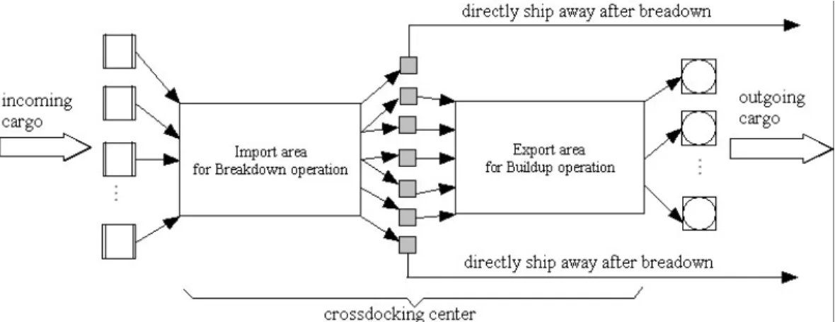
(17) Chapter 2. Problem Description. Typically, storage and order picking are the main operations of the handling activity in a warehouse. These operations are labor intensive and are expensive. Handling costs and space utilization need to be considered when working with a warehouse. Even more, warehouses need to be configured to handle equipment and an inventory management system is required to have everything under control. Crossdocking tries to reduce or eliminate these issues by reducing warehouses to purely transshipment centers where receiving and shipping are its only functions. Shipments need to expend very little time at crossdocks before being moved into the next level in the supply chain. At crossdocks, inbound trucks arrive with cargo that is sorted, consolidated, and loaded onto outbound trucks sent to manufacturing sites, retailers or even another warehouse or crossdock. In a crossdock, the customer is predetermined and there is no need for storage. The crossdock can be divided into an import area where breakdown occurs and an export area where buildup occurs. In the import area, incoming containers are broken down, and in the export area, containers are built up after consolidation, if necessary. Since incoming containers come from a number of suppliers, incoming cargo will reach the crossdock at different times. Items, including breakdowns, are then either sent away directly or sent to the export area to be loaded into outgoing containers. Outbound cargo is shipped away by vehicles with scheduled departure times. So, in this context, each incoming container has a release time and a due date and each outgoing container has a due date. This situation is shown in Figure 2.1.. 6.

(18) Figure 2.1 A crossdock flow - taken from Li et al. (2004). Each incoming (outgoing) container is processed by a breakdown (buildup) team of workers in the import (export) area. Since such teams are limited in number, scheduling teams to jobs has to be precise. Timing is extremely important for crossdocking. The idea is then to obtain a schedule to specify when to start breakdown and when to complete buildup of all cargo where the goal is to complete processing each container exactly at its due date. This is true for the purely crossdocking - JIT scheduling problem where the number of teams of workers in each side of the crossdock is a given parameter. For the optimal workers allocation for the crossdocking - JIT scheduling problem, in which the number of teams of workers in each side of the crossdock is an unknown variable that has to be determined, the costs are due to two factors: the number of teams of workers hired to do the job, and the transit storage time for cargo. Each team of workers has a fixed cost per working day, and the cargo can incur, as mentioned before, early and tardy delivery costs. The cost per working day of each team of workers is the same for both sides of the crossdock, and, as it is known, the transit storage time for cargo is minimized according to JIT scheduling. Then, the complete goal is to obtain both: the optimal number of teams of workers in each side of the crossdock and a schedule that specifies when to start breakdown and when to complete buildup of all cargo.. 7.

(19) 2.1 Literature Review.. The first study related to JIT scheduling appeared with the work done by Sidney (1977) who analyzed a scheduling problem for a single machine with earliness and tardiness penalties, considering intervals for processing the jobs, and idle times. In that paper, an earliness penalty occurs when a job starts before its target start time. Tardiness penalty occurs when a job finishes after its target due date. A job j incurs no penalty if it is processed entirely in the target interval [start timej, due datej]. The 2 author presented a polynomial time algorithm with O(n ) order for solving this. problem, where n is the number of jobs in the problem instance. Later, Lakshminarayan et al. (1978) developed a polynomial time algorithm with O(nlogn) order for solving this same problem. The following variations of JIT machine scheduling problems were studied for a single machine with a common due date with some differences: •. Large common due date (d) - the problem is called unrestricted because the scheduling decision will not be affected by the value of the due date. Bagchi et al. (1986) showed that this problem can be solved in polynomial time. •. Not large common due date (d) - Hall et al. (1991) showed that this problem is NP-complete in the ordinary sense, even for not weighted unit earliness and tardiness penalties of jobs (α = β = 1). In the same work, the authors showed that if unit earliness and tardiness penalties are job-dependent (αj, βj), the problem is NP-hard, even for a large common due date (d). Liaw (1999) proposed a branch and bound algorithm with dominance rules to minimize the sum of weighted earliness (α) and weighted tardiness (β) for a single machine scheduling problem where no machine idle time is allowed. An excellent survey of JIT scheduling for single machine can be found in Baker and Scudder (1990). They start the review with a basic model that contains symmetric. 8.

(20) penalties and a common due date, and then they add some features to this basic model to form a framework for models classification with the following characteristics: •. Linear and quadratic objective functions. •. Symmetric unit earliness and tardiness penalties (α = β), different unit earliness and tardiness penalties (α ≠ β), and job-dependent unit earliness and tardiness penalties (αj, βj). •. Common due date (d) and job-dependent due dates (dj). Job-dependent due dates (dj) complicate the problem because most of the properties of optimal schedules do not hold any longer. Garey et al. (1988) showed that the problem of finding minimal cost schedules with job-dependent due dates (dj) is NPcomplete. In many studies, release times are not considered by researchers because jobs are assumed to be ready at time 0. Mazzini and Armentano (2001) developed a constructive heuristic and an adjacent pairwise interchange heuristic to solve the problem where each job has its own release time (rj) and its own due date (dj). There is little research on JIT scheduling for parallel machines and most research done on this problem deals with a common due date (d). Few authors study this problem with job-dependent due dates (dj). Laguna and González-Velarde (1991) proposed a search heuristic for the uncommon weighted earliness penalty (αj) problem with job-dependent deadlines (mandatory dj) in parallel identical machines. Sivrikaya-Serifoglu and Ulusoy (1999) employed two genetic algorithm approaches to heuristically solve a parallel machine scheduling problem with common and unequal weighted earliness and tardiness penalties (α, β) where the due dates of the jobs are distinct (dj) and each job has its own arrival time (rj). Heady and Zhu (1998) provided a heuristic algorithm for the uncommon weighted (αj, βj) JIT scheduling problem with job-dependent due dates (dj) in a multi-machine system where processing times depend on the job-machine combination. Radhakrishnan and Ventura (2000) provided local search heuristics in the framework of the Simulated Annealing. 9.

(21) technique for the parallel machine earliness-tardiness uncommon due date (dj) sequence-dependent set-up time scheduling problem. No previous research has been done on the JIT machine scheduling characterization of the crossdocking problem, except for the one discussed in Li et al. (2004). They proposed two algorithms to solve this problem: SWOGA and LPGA. The first one uses Squeaky Wheel Optimization embedded in a Genetic Algorithm and the second one uses Linear Programming within a Genetic Algorithm. However, the work presented in this thesis considers a different metaheuristic approach applied to this problem. Besides, the source codes of our work are available for the reader. The crossdocking - JIT scheduling problem is NP-hard because if the due dates of the outgoing jobs are very large, the two phases of the problem could be processed independently (the second phase of the problem would not depend on the results of the first phase), and each phase could be reduced to the JIT scheduling problem for parallel machine with job-dependent due dates which it is known to be NP-hard, since the case for single machine is already NP-hard [Garey et al. (1988)]. Rosas (1991), Rivera (1996), and Li et al. (2004) contain a section in their works that include an excellent literature review related to JIT scheduling. On the other hand, some works related to JIT scheduling but now considering a variable number of teams of workers are referred below. This bigger problem includes the workforce allocation task whose study is varied. Abernathy et al. (1973) presented a hierarchical scheme of three phases: planning, scheduling, and allocation, to solve a nurse-staffing problem in a hospital. They formulated the planning and scheduling stages as a stochastic programming model, suggested an iterative solution procedure using random loss functions, and developed a non iterative solution procedure for a chance-constrained formulation that considers alternative operating procedures and service criteria. They made the assignment of tasks to multi-functional workers during the allocation phase. Siferd and Benton (1992) extended this hospital nurse staffing and scheduling study.. 10.

(22) Baker (1976) studied the basic mathematical models for workforce scheduling with cyclic demand for staff. Lewis et al. (1998) studied how the tasks in a fixed size office should be organized to maximize throughput when short-term reassignment of workers is difficult, costly, or restricted. Heymann et al. (2000) studied how many workers should be allocated for executing a distributed application and how to assign tasks to workers in order to maximize resource efficiency and minimize application execution time. They proposed an effective scheduling strategy that dynamically measures the execution times of tasks and uses this information to dynamically adjust the number of workers to achieve a desirable efficiency, minimizing the impact of loss of speedup. Brennan and Orwig (2000) examined conflicting approaches to work allocation in an engineering consulting firm. They proposed an analytical framework to determine whether a leveraged approach is superior to a cascaded bin packing approach for the organization’s performance. Iima and Sannomiya (2001) proposed a module type genetic algorithm to solve a modified job-shop scheduling problem with a workers allocation constraint. Campbell and Diaby (2002) used mathematical programming to model a multi-department and labor-intensive service environment problem. They proposed a heuristic based on a linear assignment approximation for allocating cross-trained workers to multiple departments at the beginning of a shift. They considered the re-assignment of tasks to workers within the shifts. Gomar et al. (2002) developed a linear programming model to help optimize the multi-skilled workforce assignment and allocation process in a construction project. Tharmmaphornphilas and Norman (2004) proposed a quantitative method based on mathematical programming to obtain a proper job rotation interval length in a work setting in order to reduce worker fatigue and injuries and improve the quality of the job. Corominas et al. (2004) solved a problem of allocating types of tasks to the multifunctional workers of a service center over a time horizon assuming equal efficiency for all of the members of the staff.. 11.

(23) No previous research has been done on the machine characterization of the optimal workers allocation for the crossdocking - JIT scheduling problem. It was previously shown that the purely crossdocking - JIT scheduling problem is NPhard. Therefore, the optimal workers allocation for the crossdocking - JIT scheduling problem is NP-hard as well.. 2.2 Relationship of the Problem with Machine Scheduling.. The crossdocking - JIT scheduling problem described before can be modeled naturally as a machine scheduling problem as follows: each incoming container can be thought of as a job which has a release time after which it can be processed, a due date, and a processing time. Each outgoing container can be thought of as a job which has a number of source containers or predecessors which feed it, a due date, and a processing time. These incoming/outgoing jobs are processed by teams of workers which can be thought of as machines. These machines handling incoming/outgoing. cargo. are. parallel. because. they. are. able. to. operate. simultaneously. The parameters used in this model are: ri - release time after which incoming container i can be broken down di - due date for incoming container i pi - processing time required to break down incoming container i Sij - the ith source of outgoing container j. Outgoing container j is built from Kj different incoming containers Dj - due date of outgoing container j Pj - processing time required to build up outgoing container j n - number of incoming containers. 12.

(24) m - number of breakdown teams N - number of outgoing containers M - number of buildup teams α - penalty for unit time earliness β - penalty for unit time tardiness For the purposes of this project, it is assumed that n > m, and N > M (only for the purely crossdocking - JIT scheduling problem where m and M are given parameters). The number of jobs n and N do not have to be equal, and the number of teams m and M do not have to be equal either. Another note related to the problem is the representation of the Sij matrix given by the n incoming containers and the N outgoing containers. The cargo of one incoming container might be loaded in zero or more outgoing containers, and the cargo built up in one outgoing container might come for one or more incoming containers. If the cargo of one incoming container is loaded in zero outgoing containers it means that the cargo is directly shipped away after breakdown. Other assumptions to be considered for this project are: •. Teams are identical. •. Teams are available at time 0. •. Teams are 100% reliable (machines do not get out of order). •. A team can not process more than one job at the same time. •. There are no preemptions in the scheduling, this is, once a team starts to process a job, this job has to be finished before the team can start processing another job. •. Containers and teams have infinite capacity (the number of handled items can be any number). •. All the cargo arriving to the crossdock leaves the crossdock. 13.

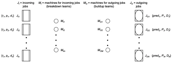
(25) •. Distribution times for the jobs inside the crossdock are already included in their corresponding processing times. •. The horizon of the process is one working day. In the problem context, suppliers do not want to expend too much time in the crossdock because it is very likely that they have to deliver more cargo to some other customers and they do not want to be late. On the other hand, suppliers should not be early because the crossdock authorities do not want to have their cargo too much time inside the crossdock to avoid inventory and it is very likely that they need that space for some other suppliers. This agrees with the JIT scheduling philosophy. Incoming jobs are described by JI = {JI1, JI2, …, JIn} and outgoing jobs are described by JO = {JO1, JO2, …, JON}. Breakdown teams are described by MI = {MI1, MI2, …, MIm} and buildup teams are described by MO = {MO1, MO2, …, MOM}. Jobs in JI are processed only by teams in MI, and jobs in JO are processed only by teams in MO. A job JIi ∈ JI is described by {ri, pi, di}, where ri, pi, di denote its release time, processing time, and due date, respectively. A job JOj ∈ JO is described by {predj, Pj, Dj}, where Pj and Dj denote its processing time and due date, respectively, and predj describes its predecessors, all belonging to JI. Actually, predj represents a column of the Sij matrix. A representation of the sources or predecessors of outgoing containers and the Sij matrix is shown in Figure 2.2.. Kj sources or predecessors of outgoing container j. first predecessor of outgoing container j. b). outgoing container j. Sij =. 1 2 0 1 1 0 1 1 1 0 K1 = 3 K2 = 2. outgoing container j. second predecessor of outgoing container j. • • •. incoming container i. a). last predecessor of outgoing container j. 1 2 3 4. Figure 2.2 a) A representation of the sources or predecessors of an outgoing container j; b) An example of an Sij matrix with 4 incoming containers and 2 outgoing containers. 14.

(26) Earliness and tardiness penalties of a job JIi are defined by ei = max{0, di - ci} and ti = max{0, ci - di}, respectively, where ci represents the incoming job’s finish time. Earliness and tardiness penalties of a job JOj are defined by Ej = max{0, Dj - Cj} and Tj = max{0, Cj - Dj}, respectively, where Cj represents the outgoing job’s finish time. The objective of the problem is to find a schedule that minimizes the total penalty. Figure 2.3 shows a more detailed view of Figure 2.1 and it represents a summary of the whole situation. JI = incoming jobs. MI = machines for incoming jobs (breakdown teams). MO = machines for outgoing jobs (buildup teams). JO = outgoing jobs. {r1, p1, d1} JI1. JO1 {pred1, P1, D1}. {r2, p2, d2} JI2. • • •. MI1. MO1. MI2. MO2. • • •. JO2 {pred2, P2, D2}. • • • MIm. MOM. • • •. {rn, pn, dn} JIn. JON {predN, PN, DN}. Figure 2.3 A more detailed flow for the crossdocking - JIT scheduling problem. In Figure 2.3, each incoming job represents a container coming from a company like Pepsico, the Coca-Cola Company, Bimbo, Cuauhtémoc-Moctezuma Beer Company, Kraft, Kimberly-Clark, among many others. Each one of these companies’ trucks contains several products that are going to be spread out through several locations like, i.e. in the Monterrey city area, Wal-Mart Las Torres, Wal-Mart Valle Oriente, Wal-Mart Lincoln, etc. The Wal-Mart example is used because crossdocking has received much attention as a result of the commercial success of large transshipments in this company [Gue (2001)]. In the same Figure 2.3, predj means that job JOj contains cargo from Kj different incoming containers or jobs. As mentioned before, cargo is processed in two phases: breakdown and buildup. Precedence relationships exist between these phases in the following sense: each incoming container i must be broken down before an outgoing container j can. 15.

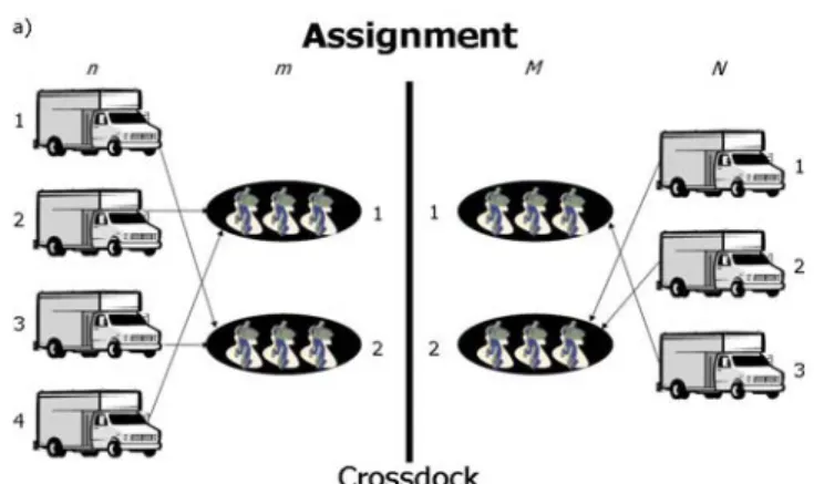
(27) commence to be built up if cargo items in container j come from container i. In other words, a container can start buildup only if all its source containers have been broken down in order to have all its items correctly loaded. Buildup should not start before complete breakdown because it could be possible to have the heaviest items loaded in the top of the container. This situation is part of another problem known as the Bin Packing Problem [Coffman (1976), Baase (1991), Hochbaum (1997), Horowitz et al. (1998), Cormen et al. (2001)] whose study is beyond the scope of this work. It is known that there are no release times for buildup. It is also known that buildup can not commence in outgoing container j until all its cargo predecessors have been broken down. So, it is possible to define the state variable Rj as follows: the completion time of last incoming container i broken down which contains cargo for outgoing container j, or Rj = max{ci}, i = first predecessor of outgoing container j, …, last predecessor of outgoing container j. Rj can be seen as the release time of the outgoing container j, however, its value depends on the current schedule. In summary, the crossdocking - JIT scheduling problem can be viewed as a twophase parallel machine scheduling problem. Also, each phase of the problem can be seen as an assignment - scheduling problem (the sequencing activity is implicitly included in the scheduling activity), according to Figure 2.4.. 16.

(28) containers (jobs). teams of workers (machines). Assignment. Scheduling. Figure 2.4 Inbound or outbound area of the crossdocking - JIT scheduling problem seen as an assignment scheduling problem. The sequencing part of the problem shown in Figure 2.4 can also be seen as a Traveling Salesman Problem (TSP) [Lawler et al. (1985)]. So, the whole picture of the Figure 2.4 can be viewed as a Vehicle Routing Problem (VRP) [Crainic and Laporte (1998)]. The optimal workers allocation for the crossdocking - JIT scheduling problem can be modeled as a machine scheduling problem just exactly in the same way as it is done for the purely crossdocking - JIT scheduling problem. However, in this bigger problem the incoming and outgoing jobs (n and N, respectively) are processed by an unknown number of teams of workers (m and M) which can also be thought of as machines. The assumptions to be considered and most of the parameters used for the model for this bigger problem are the same mentioned for its sub-problem, but the number of breakdown teams (m) and the number of buildup teams (M) are not. 17.

(29) considered parameters any more, and the cost of a team hired (h) is a new parameter that has to be considered. As mentioned before, the number of teams hired to do the breakdown (m) and the buildup (M) is unknown. Obviously, in both cases the minimum number of teams hired is 1 and the maximum number of teams hired for the breakdown is the total number of incoming jobs (n) and for the buildup is the total number of outgoing jobs (N). As said earlier, the number of jobs n and N do not have to be equal, and the number of teams m and M do not have to be equal either.. 2.3 Model for the Problem.. Crossdocking - JIT scheduling problem As the crossdocking - JIT scheduling problem described above can be seen as a machine scheduling problem, it is possible to formulate it with the following integer programming model taken from Li et al. (2004):. Decision variables yik = 1 if incoming container i is processed by breakdown team k and 0 otherwise, for i = 1, …, n, k = 1, …, m Yjk = 1 if outgoing container j is processed by buildup team k and 0 otherwise, for j = 1, …, N, k = 1, …, M Iijk = 1 if incoming containers i and j are both processed by breakdown team k and i precedes (not necessarily immediately) j, and 0 otherwise, for i, j = 1, …, n, i ≠ j, k = 1, …, m Jijk = 1 if outgoing containers i and j are both processed by buildup team k and i precedes (not necessarily immediately) j, and 0 otherwise, for i, j = 1, …, N, i ≠ j, k = 1, …, M 18.

(30) ci - completion time of incoming container i, i = 1, …, n Cj - completion time of outgoing container j, j = 1, …, N Variables yik and Yjk represent assignment variables, Iijk and Jijk represent sequencing variables, and ci and Cj represent scheduling variables. The values assigned to the assignment variables and to the scheduling variables represent a specific solution for the problem.. State variables: their values depend on the current built schedule ei - earliness of incoming container i, i = 1, …, n Ej - earliness of outgoing container j, j = 1, …, N ti - tardiness of incoming container i, i = 1, …, n Tj - tardiness of outgoing container j, j = 1, …, N. Objective function n. ∑ (α e. Minimize. i. + β ti ) +. i =1. ∑ (α E N. j. + βT j ). j =1. Constraints For job to team uniqueness - each job must be processed by exactly one team: (1). m. ∑y k =1. (2). ik. = 1 , i = 1, …, n (breakdown area). M. ∑Y k =1. jk. = 1 , j = 1, …, N (buildup area). For job precedence relationships: (3). yik + yjk - (Iijk + Ijik) ≤ 1 (breakdown area). 19.

(31) (4). 2(Iijk + Ijik) - yik - yjk ≤ 0 (breakdown area) i, j = 1, …, n, i < j, k = 1, …, m. These two previous groups of constraints come from a transformation of the following relationships: yik + yjk = 2 Ù Iijk + Ijik = 1 (jobs i and j are processed by the same team) yik + yjk ≤ 1 Ù Iijk + Ijik = 0 (jobs i and j are not processed by the same team) i, j = 1, …, n, i < j, k = 1, …, m A similar reasoning is used for the outgoing containers, obtaining: (5). Yik + Yjk - (Jijk + Jjik) ≤ 1 (buildup area). (6). 2(Jijk + Jjik) - Yik - Yjk ≤ 0 (buildup area) i, j = 1, …, N, i < j, k = 1, …, M. For sufficient time between jobs on the same team - if job i precedes job j, there must be enough time between them for job j to be completed: (7) (8). ci ≤ (cj - pj) + G(1 - Iijk), i, j = 1, …, n, i ≠ j, k = 1, …, m (breakdown area) Ci ≤ (Cj - Pj) + G(1 - Jijk), i, j = 1, …, N, i ≠ j, k = 1, …, M (buildup area). where G is a nonzero real number such that G ≥ max{f(x) | x ∈ D} and f : D Æ R for some D, δ ∈ {0, 1}. Then, for each δ ∈ {0, 1} and x ∈ D, the following are equivalent:. •. δ = 0 Æ f(x) ≤ 0. •. f(x) - G·δ ≤ 0. This binary variables reduction lemma is better explained in Sierksma (2001). Since it is not easy to know the exact value that satisfies the conditions mentioned above, Li et al. (2004) recommend, for practical purposes, to use a big value for G. They used G = 10,000 for their runs. The rest of the groups of constraints that complete the model are: (9). ci - ri ≥ pi, i = 1, …, n (breakdown area) 20.

(32) (10). Cj - ci ≥ Pj, j = 1, …, N, i = first predecessor of outgoing container j, …, last predecessor of outgoing container j (buildup area) (11) (12). ci - di = ti - ei, i = 1, …, n (breakdown area) Cj - Dj = Tj - Ej, j = 1, …, N (buildup area) yik ∈ {0, 1}, i = 1, …, n, k = 1, …, m Yjk ∈ {0, 1}, j = 1, …, N, k = 1, …, M. Iijk ∈ {0, 1}, i, j = 1, …, n, i ≠ j, k = 1, …, m Jijk ∈ {0, 1}, i, j = 1, …, N, i ≠ j, k = 1, …, M ci, ei, ti ∈ Z+ (nonnegative integer numbers), i = 1, …, n Cj, Ej, Tj ∈ Z+ (nonnegative integer numbers), j = 1, …, N The group of constraints (9) enforces release times in the breakdown area. The group of constraints (10) specifies that an outgoing container can start buildup only if all its source containers have been broken down. The groups of constraints (11) and (12) specify each job’s earliness and tardiness in the breakdown area and the buildup area, respectively. This model contains:. •. A total of variables (including state variables) equal to n 2 m + N 2 M + 3(n + N ) , from which:. •. o. n 2 m + N 2 M are binary variables and 3(n + N ) are integer variables. o. n 2 m + N 2 M + n + N are decision variables and 2(n + N ) are state variables N. A total of constraints equal to 3n + 2 N + 2(n 2 − n)m + 2( N 2 − N ) M + ∑ K j , where j =1. N. N ≤ ∑ K j ≤ nN j =1. 21.

(33) •. A total of non-empty cells in the technological coefficients matrix (see Appendix 1) N. equal to 4n + 3 N + nm + NM + 7(n 2 − n)m + 7( N 2 − N ) M + 2∑ K j j =1. The technological coefficients matrix is sparse because the total of non-empty cells is too small with respect to the total of cells in that matrix. This total of cells is computed multiplying the total of variables times the total of constraints. This situation can be noticed in Table 2.1 n. m. N. M. Total of variables. 4 5 10 15 20 24. 2 3 2 3 8 11. 3 4 11 14 18 25. 2 3 3 2 7 12. 71 150 626 1154 5582 13983. Total of Total of constraints non-empty cells Min case Max case Min case Max case 297 315 93 102 739 771 219 235 3718 3916 1083 1182 7161 7553 2075 2271 36730 37414 10478 10820 93689 94839 26691 27266. Total of Percentage of cells occupation Min case Max case Min case Max case 6603 7242 4.5% 4.3% 32850 35250 2.2% 2.2% 677958 739932 0.5% 0.5% 2394550 2620734 0.3% 0.3% 58488196 60397240 0.1% 0.1% 373220253 381260478 0.0% 0.0%. Table 2.1 Percentage of occupation of the technological coefficients matrix for different crossdocking - JIT scheduling problem instances. It can be seen in Table 2.1 that the percentage of occupation of the technological coefficients matrix tends to zero as the problem instance grows.. Optimal Workers Allocation for the crossdocking - JIT scheduling problem The integer programming model for the optimal workers allocation for the crossdocking - JIT scheduling problem presented below is very similar to the one shown for its sub-problem, the purely crossdocking - JIT scheduling problem. It is possible to formulate it using the machine scheduling notation as follows:. Decision variables yik = 1 if incoming container i is processed by breakdown team k and 0 otherwise, for i = 1, …, n, k = 1, …, n 22.

(34) Yjk = 1 if outgoing container j is processed by buildup team k and 0 otherwise, for j = 1, …, N, k = 1, …, N Iijk = 1 if incoming containers i and j are both processed by breakdown team k and i precedes (not necessarily immediately) j, and 0 otherwise, for i, j = 1, …, n, i ≠ j, k = 1, …, n Jijk = 1 if outgoing containers i and j are both processed by buildup team k and i precedes (not necessarily immediately) j, and 0 otherwise, for i, j = 1, …, N, i ≠ j, k = 1, …, N ci - completion time of incoming container i, i = 1, …, n Cj - completion time of outgoing container j, j = 1, …, N mk = 1 if breakdown team k is hired and 0 otherwise, for k = 1, …, n Mk = 1 if buildup team k is hired and 0 otherwise, for k = 1, …, N Variables yik and Yjk represent assignment variables, Iijk and Jijk represent sequencing variables, ci and Cj represent scheduling variables, and mk and Mk represent machines variables. The values assigned to the assignment variables, scheduling variables and machines variables represent a specific solution for the problem.. State variables: their values depend on the current built schedule ei - earliness of incoming container i, i = 1, …, n Ej - earliness of outgoing container j, j = 1, …, N ti - tardiness of incoming container i, i = 1, …, n Tj - tardiness of outgoing container j, j = 1, …, N. Objective function. 23.

(35) n. Minimize. ∑ (α e i =1. i. + β ti ) +. ∑ (α E N. j =1. j. + βT j )+ h∑ mk + h∑ M n. N. k =1. k =1. k. Constraints (1). n. ∑y. ik. = 1 , i = 1, …, n (breakdown area). k =1. (2). N. ∑Y k =1. jk. = 1 , j = 1, …, N (buildup area). (3). yik + yjk - (Iijk + Ijik) ≤ 1 (breakdown area). (4). 2(Iijk + Ijik) - yik - yjk ≤ 0 (breakdown area) i, j = 1, …, n, i < j, k = 1, …, n. (5). Yik + Yjk - (Jijk + Jjik) ≤ 1 (buildup area). (6). 2(Jijk + Jjik) - Yik - Yjk ≤ 0 (buildup area) i, j = 1, …, N, i < j, k = 1, …, N. (7). ci ≤ (cj - pj) + G(1 - Iijk), i, j = 1, …, n, i ≠ j, k = 1, …, n (breakdown area). (8). Ci ≤ (Cj - Pj) + G(1 - Jijk), i, j = 1, …, N, i ≠ j, k = 1, …, N (buildup area) (9). (10). ci - ri ≥ pi, i = 1, …, n (breakdown area). Cj - ci ≥ Pj, j = 1, …, N, i = first predecessor of outgoing container j, …, last predecessor of outgoing container j (buildup area) (11) (12) (13) (14). ci - di = ti - ei, i = 1, …, n (breakdown area) Cj - Dj = Tj - Ej, j = 1, …, N (buildup area). mk - yik ≥ 0, i = 1, …, n, k = 1, …, n (breakdown area) Mk - Yjk ≥ 0, j = 1, …, N, k = 1, …, N (buildup area) yik ∈ {0, 1}, i = 1, …, n, k = 1, …, n. 24.

(36) Yjk ∈ {0, 1}, j = 1, …, N, k = 1, …, N Iijk ∈ {0, 1}, i, j = 1, …, n, i ≠ j, k = 1, …, n Jijk ∈ {0, 1}, i, j = 1, …, N, i ≠ j, k = 1, …, N mk ∈ {0, 1}, k = 1, …, n Mk ∈ {0, 1}, k = 1, …, N + ci, ei, ti ∈ Z (nonnegative integer numbers), i = 1, …, n + Cj, Ej, Tj ∈ Z (nonnegative integer numbers), j = 1, …, N. All groups of constraints were previously explained, except for the new groups of constraints (13) and (14) which specify that a job can only be assigned to a team of workers that has been hired. Again, for the group of constraints (7) and (8), it is recommended, for practical purposes, to use a big value for G since it is not easy to know the exact value for G that satisfies them. We used G = 100,000 for the experiments. This value for G is bigger than the one mentioned for the previous model because the model of this bigger problem considers the costs due to the number of teams of workers hired in each side of the crossdock. For the cost of a team hired we used a value of h = 1,000. This model contains:. •. A total of variables (including state variables) equal to n 3 + N 3 + 4(n + N ) , from which:. •. o. n 3 + N 3 + n + N are binary variables and 3(n + N ) are integer variables. o. n 3 + N 3 + 2(n + N ) are decision variables and 2(n + N ) are state variables N. A total of constraints equal to 3n + 2 N − (n 2 + N 2 ) + 2(n 3 + N 3 ) + ∑ K j , where j =1. N. N ≤ ∑ K j ≤ nN j =1. 25.

(37) •. A total of non-empty cells in the technological coefficients matrix equal to N. 4n + 3 N − 4(n 2 + N 2 ) + 7(n 3 + N 3 ) + 2∑ K j j =1. 26.

(38) Chapter 3. Heuristics and Metaheuristics. One of the goals of this project is to create an algorithm able to solve the optimal workers allocation for the crossdocking - JIT scheduling problem described in Chapter 2. As mentioned before, this problem is NP-hard, therefore, the use of heuristics and metaheuristics to obtain a good feasible solution for big instances is an important option to consider.. 3.1 Heuristics.. Given the difficulty to obtain an optimal solution by an exact method, i.e. using the simplex method [Murty (1983), Bazaraa et al. (1990), Dantzig and Thapa (2003)] or a branch and bound algorithm [Horowitz et al. (1998), Neapolitan and Naimipour (1998)], for a group of important combinatorial optimization problems when dealing with big instances, some series of algorithms that provided near optimal feasible solutions in a reasonable processing time started to appear in the last decades. These kinds of algorithms were denominated heuristics. In this context, “near optimal” and “reasonable” can be considered as subjective terms. The word "heuristic" derives from the Greek "heuriskein," which means "to discover", however, this meaning might be changed for the meaning “to search” because that is what heuristics actually do in practice. Polya (1957) was one of the first authors in mentioning the word heuristic. He claimed: “heuristics are methods of solution that aims at generality, at the study of procedures which are independent of the subject-matter and apply to all sorts of. 26.

(39) problems”. Zanakis and Evans (1981) defined the heuristics as “simple procedures, often guided by common sense, that are meant to provide good but not necessarily optimal solutions to difficult problems, easily and quickly”. Another definition of heuristic is given by Adam and Ebert (1991) as a “set of methods and principles whose result is a satisfactory solution of the problem obtained by using simple criteria that allow correctly identifying good decisions”. Their lack of mathematical rigor and the easiness of their designs have made the heuristics gain acceptance by many practitioners who are interested in a useful tool to obtain a quick solution for complex problems in a way that they can understand. On the other hand, one of the major disadvantages of heuristics is that, generally, the quality of their solutions can not be known. Even though there are many advantages when using a heuristic, if an optimal algorithm can be used effectively to solve a problem, this last action must be done. Zanakis and Evans (1981) explained why and when the use of heuristics is desirable and advantageous.. 3.2 Metaheuristics.. In their original definition, “metaheuristics are solution methods that orchestrate an interaction between local improvement procedures and higher level strategies to create a process capable of escaping from local optima and performing a robust search of a solution space”. Over time, these methods have also included any procedures that employ strategies for overcoming the trap of local optimality in complex solution spaces, specially those procedures that use one or more neighborhood structures as a mean of defining admissible moves to transition from one solution to another, or to build or destroy solutions in constructive and destructive processes [Glover and Kochenberger (2003)]. Gendreau (2002) defined a metaheuristic as a “general strategy for guiding and controlling inner heuristics”. Metaheuristics provide general frames that allow the creation of new hybrids by combining different concepts derived from classic heuristics, artificial intelligence,. 27.

(40) biological evolution, neural systems, and statistical mechanics, among others. A number of tools and mechanisms that have emerged from the creation of metaheuristic methods have proved to be so effective that metaheuristics have lately become the preferred method used for solving many types of complex problems, especially combinatorial problems [Glover and Kochenberger (2003)]. Metaheuristics can be classified according to their use of memory: metaheuristics with memory and metaheuristics without memory. Unlike the metaheuristics without memory, the metaheuristics with memory contain structures that retain information about decisions previously taken, allowing that way a kind of learning. Commonly, Tabu Search and Scatter Search are classified as metaheuristics with memory while Simulated Annealing and GRASP are considered metaheuristics without memory [De Alba (2004)]. Of course, some metaheuristics that usually do not make use of memory to solve problems can be adapted to make use of it for a specific purpose. Heuristics and metaheuristics are important approaches used in the operations research field and, in particular, in the combinatorial optimization field, which includes most of the interesting scheduling problems. Over the last years, these approaches have been used to solve complex problems in several applications, including NP-hard scheduling applications [Crainic and Laporte (1998)]. Very general methods having a wide range of applicability are typically weak with respect to their performance. Genetic Algorithms and Neural Networks tend to belong to this category. Problem specific methods achieve a highly efficient performance but with little use in other problem domains. Tabu Search and Simulated Annealing can be counted as examples of this category. Regardless of the category, heuristics and metaheuristics can be viewed as tools for searching a space of feasible alternatives in order to find a good solution within reasonable time limitations, but without any guarantee of optimality [Blazewicz et al. (2001)]. An excellent description and classification of heuristics and metaheuristics are given in Díaz et al. (1996). Glover and Kochenberger (2003) present research done by several renowned authors in the field of the metaheuristics.. 28.

(41) To solve the problem described in Chapter 2 an approach based on a combination of two metaheuristics, GRASP and Tabu Search, is proposed. Each one of these metaheuristics is explained next. 3.2.1 GRASP.. Greedy Randomized Adaptive Search Procedure (GRASP) was developed by Feo and Resende (1989) to study a complex set covering problem. In its basic version, GRASP is a multi-start or iterative method that consists of two phases at each iteration: a constructive phase whose result is a feasible and good but not necessarily optimal solution, and a local search procedure, during which, neighborhoods of the solution are examined until a local optimum is attained. The construction phase is based on the idea that a variety of good solutions can be generated by an “intelligent randomization” of the selection step of a greedy heuristic. These solutions are then passed to an exchange procedure that searches for local improvements. The iterations proceed, keeping the best solution found, until a stopping criterion is reached [Laguna and González-Velarde (1991)]. Then, GRASP has two main parameters: one related to the stopping criterion and another related to the amount of “randomization” allowed in the selection step of a greedy heuristic. This last parameter is often called α. The case α = 0 corresponds to a pure greedy algorithm while α = 1 is equivalent to a completely random algorithm. Figure 3.1 shows a basic GRASP pseudo-code taken from Resende and Ribeiro (2001). For this particular case, the stopping criterion of the procedure is the maximum number of iterations while the parameter α is not mentioned. procedure GRASP( Max_Iterations ) Best_solution Å ∞ or -∞; // minimization or maximization problem for i = 1, …, Max_Iterations do Solution Å Greedy_Randomized_Construction(); Solution Å Local_Search( Solution ); Update_Solution( Solution , Best_Solution ); end for; return Best_solution; end GRASP.. 29.

(42) Figure 3.1 Pseudo-code for a basic GRASP procedure. Other pseudo-codes for a basic GRASP are shown in Díaz et al. (1996) and in Resende and González-Velarde (2003). Unlike the rest of the metaheuristics, which operate over previously obtained solutions, GRASP is a constructive method that focus on building high-quality solutions for further processing in order to get better results. At each step of the construction phase, a substructure is added to a partial solution, initially empty, until a complete solution is found. Each one of the words that form the acronym GRASP characterizes one of the components of this metaheuristic. At each iteration of the construction phase, GRASP maintains a set of candidate elements that can be feasibly incorporated to the partial solution under construction. All candidate elements are evaluated according to a greedy function in order to select the next element to be added to the construction. This greedy function usually represents the marginal increase in the cost function from adding the element to the partial solution. The evaluation of the elements is used to create a restricted candidate list (RCL) which consists of the best elements, i.e. those whose incorporation to the current partial solution results in the smallest incremental costs (for a minimization problem) -this is the greedy aspect of the method-. The element to be added into the partial solution is randomly selected from those in the RCL -this is the random aspect of the metaheuristic-. Once the selected element is added to the partial solution, the RCL is updated and the incremental costs are recalculated -this is the adaptive aspect of the metaheuristic-. The previous high-level description of the components of the GRASP technique was taken from Resende and Ribeiro (2001) and from Laguna and Martí (2003). The immediate GRASP strategy predecessor is the semi-greedy heuristic proposed by Hart and Shogan (1987), which is also a multi-start approach based on greedy randomized constructions, but without local search. An older background of the GRASP technique can be found in Lin and Kernighan (1973).. 30.

(43) The solutions generated by a greedy randomized construction are not necessarily optimal, even with respect to simple neighborhoods. The local search phase usually improves the constructed solution. A local search algorithm works in an iterative fashion by successively replacing the current solution by a better solution found in the neighborhood of the current solution. This procedure can be done during the construction phase or at the end of it. Local search is very important for the GRASP technique because it is useful when searching locally optimal solutions in promising regions of the solutions space. GRASP is based on the premise that good and diverse initial solutions play an important role in the success of local search methods. The effectiveness of a local search procedure depends on several aspects, such as the neighborhood structure, the neighborhood search techniques, the speed of evaluation of the objective function of neighbor solutions, and the initial solution. The construction phase plays a critical role with respect to providing high-quality starting solutions for the local search. Simple neighborhoods structures are usually used. The neighborhood search may be implemented using either a best-improving or a first-improving strategy. In the case of the best-improving strategy, all neighbors are examined and the current solution is replaced by the best neighbor. In the case of the first-improving strategy, the current solution moves to the first neighbor whose cost function value is strictly less than that of the current solution (for a minimization problem). The first phase (construction) of the GRASP metaheuristic constitutes the core of this technique. The way in which the second phase (local search) of this procedure is done varies from methods that explore simple neighborhoods through more sophisticated procedures. Very often, a local search ends in a locally optimal solution. To escape from these local optima, several strategies have been suggested, i.e. the use of other metaheuristics as an improvement procedure. Actually, GRASP hybridizations with other metaheuristics that use GRASP results as initial solutions are common. Actually, for the local improvement phase of the work under study in this thesis, the Tabu Search algorithm with the best-improving strategy is used. 31.

(44) 3.2.2 Tabu Search.. According to Glover and Laguna (1997), “Tabu Search (TS) is a metaheuristic procedure that guides a local heuristic search algorithm to explore the solution space beyond local optimality”. The local procedure is a search that uses an operation called “move” to define the neighborhood of any given solution. TS is based on the premise that problem solving, in order to qualify as intelligent, must incorporate “adaptive memory” and “responsive exploration”. The adaptive memory feature of TS allows the implementation of procedures that are capable of searching the solution space economically and effectively. Since local choices are guided by information collected during the search, TS contrasts with memory-less designs that heavily rely on random processes that implement a form of sampling, i.e. GRASP. Memory-based strategies are then the hallmark of TS approaches. Actually, TS is perhaps the metaheuristic procedure that employs memory in the most strategic and direct way. On the other hand, the emphasis on responsive exploration in TS derives from the supposition that a bad strategic choice can yield more information than a good random choice. In a system that uses memory, a bad choice based on strategy can provide useful clues about how the strategy may be profitably changed. TS is concerned with finding new and more effective ways of taking advantages of the mechanisms associated with both elements: adaptive memory and responsive exploration. These two elements of the TS procedure have several important characteristics which are summarized in Table 4.2 of Díaz et al. (1996). This previous high-level description of TS was taken from Glover and Laguna (1997) and from Laguna and Martí (2003). TS was formally proposed by Glover (1986), but its basic form is founded on some previous ideas proposed by himself [Glover (1977)], including elements like short. 32.

(45) term memory to prevent the reversal of recent moves, and longer term frequency memory to reinforce attractive components. The basic principle of TS is to pursue local search whenever it encounters a local optimum by allowing non-improving moves. Cycling back to previously visited solutions is prevented by the use of “memories”, called “tabu lists”, which record the recent history of the search. Gendreau (2002) considered TS as an extension of classical local search procedures. In fact, he mentioned that TS can be seen as simply the combination of local search with short-term memories. According to him, the two first basic elements of any TS heuristic are the definition of its “search space” and its “neighborhood structure”. The search space of a TS heuristic is simply the space of all possible solutions that can be considered (visited) during the search. The neighborhood of the current solution S, denoted by N(S), is a subset of the search space defined by the solutions obtained by applying a single local transformation to S. In general, for any specific problem, there are many more possible (an even attractive) neighborhood structures than search space definitions. This follows from the fact that there may be several feasible neighborhood structures for a given definition of the search space. Choosing a search space and a neighborhood structure is by far the most critical step in the design of any TS heuristic. Figure 3.2 shows basic TS pseudo-code taken from Pinedo (2002). In this particular case, the pseudo-code is applied to a scheduling problem and the stopping criterion of the procedure is the maximum number of iterations allowed.. 33.

(46) procedure Tabu-Search( S 1 , Max_Iterations ) Step 1: Set k = 1 Set S 0 = S 1 Step 2: Select a candidate schedule S c from the neighborhood of S k If the move S k Æ S c is prohibited by a mutation on the tabu-list then Set S k+1 = S k Go to Step 3 If the move S k Æ S c is not prohibited by any mutation on the tabu-list then Set S k+1 = S c Enter reverse mutation at the top of the tabu-list Push all other entries in the tabu-list one position down Delete the entry at the bottom of the tabu-list If Value(S c ) < Value(S 0 ) then Set S 0 = S c Step 3: Increment k by 1 If k = Max_Iterations then Stop Otherwise Go to Step 2 Figure 3.2 Pseudo-code for a basic Tabu Search procedure. It is interesting to note that in the same year that TS appeared, a similar approach named steepest ascent / mildest descent was proposed by Hansen (1986). However, in the traditional steepest ascent / mildest descent optimization method, the search stops when the value of the objective function evaluated in a solution S is not better that the obtained value in the previous iteration, this is, when a local optimum has been found. To avoid this, TS keeps exploring solutions, even non-improving ones. GRASP and TS metaheuristics are also mentioned in the next chapters, which explain the approach used to solve the problem under study.. 34.

(47) Chapter 4. Solution Approach for the Crossdocking - Just in Time Scheduling Problem. This chapter deals with the solution approach for the problem described in Chapter 2 when the number of teams of workers in each side of the crossdock is fixed and known (m and M). This is called the crossdocking - JIT scheduling problem and it represents a sub-problem (or a particular case) of the problem under study in this thesis work. This sub-problem is, as mentioned before, NP-hard.. 4.1 Solution Form.. To solve this problem it is necessary, for the inbound area, to have each one of the n incoming jobs assigned in a position in one of the m breakdown machines and a completion time. Two notes can be cited with regard to this statement: •. The use of a machine has no fixed cost; then, the model will make use of all of the available machines because that way it is easier to accommodate the jobs in order to obtain better results. It is convenient to remember that n > m and N > M. •. Once the completion time for a job is obtained, its earliness and tardiness penalties are directly obtained. Using a notation similar to the one used in Laguna and González-Velarde (1991), the incoming schedule, SI, has the form: SI = {πI, cI} where: 35.

(48) •. πI = {πI1, πI2, …, πIm} is the assignment of the n incoming jobs to the m breakdown machines. •. cI is the set of completion times for the n incoming jobs. where πIk represents the sequence in which the nk incoming jobs assigned to machine k will be processed. This πIk sequence has the following form: πIk = {πIk(1), πIk(2), …, πIk(nk)} where πIk(i) is the index of the incoming job in position i on machine k. A similar reasoning and representation is used for the outbound area and its outgoing schedule, SO. As mentioned in Chapter 1, the development of a computer program that solves the integer programming model developed by Li et al. (2004) and the development of a metaheuristic algorithm to find good solutions for different problem instances are two important tasks to consider in the project. These tasks are mentioned in the following two sections of this chapter.. 4.2 Exact Method of Solution.. Our solution of the integer programming model for the crossdocking - JIT scheduling problem developed by Li et al. (2004) is obtained through a computer program that makes use of the ILOG CPLEX 9.1 library. The results obtained by this program are compared to the results obtained by their program (which also uses the ILOG CPLEX library) for the 16 problem instances presented in their work. Obviously, the objective values shown by both versions must be the same when both algorithms reach the optimal value. The code of the computer program is easily done once the integer model is obtained. It is necessary just to follow the coding conventions mentioned in the ILOG CPLEX 9.1 User’s Manual. ILOG CPLEX search for solutions in nodes trees created according to the model. 36.

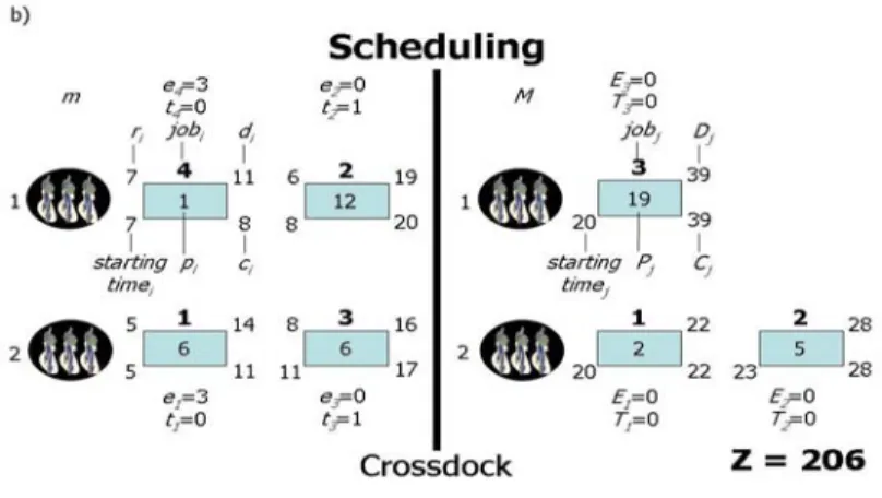
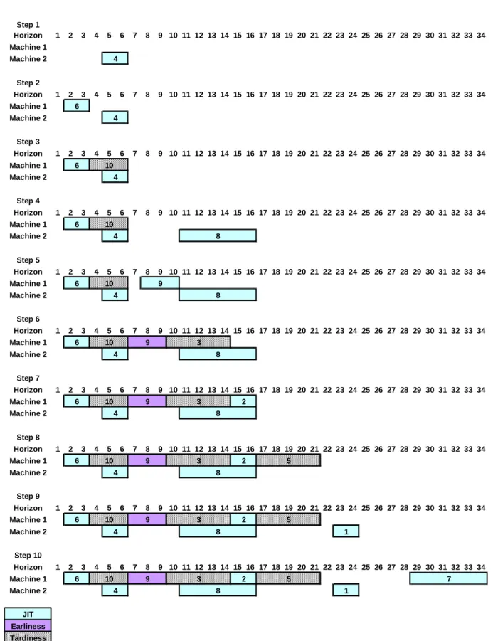
(49) defined. So, different orders in the definitions of variables and/or constraints might create different search trees (and very likely different solutions if the computer runs out of memory before reaching the optimal solution). Figure 4.1 shows the output given by the exact method algorithm for the following small problem instance. This problem instance creates an MIP with 71 variables and 99 constraints which can be seen in Appendix 2. n m N M α ß G. = 4 = 2 = 3 = 2 = 1 = 100 = 10000. 1 2 3 4. r 5 6 8 7. p 6 12 6 1. d 14 19 16 11. 1 2 3. P 2 5 19. D 22 28 39. S 1 2 3 4. 1 2 3 0 1 1 1 1 1 1 0 1 1 1 0 K 1 =3 K 2 =3 K 3 =3. Table 4.1 Input data for a crossdocking - JIT scheduling problem instance with 4 incoming jobs and 2 breakdown machines, and 3 outgoing jobs and 2 buildup machines. 37.