An analytical methodology to derive power models based on hardware and software metrics

Texto completo

(1)Noname manuscript No. (will be inserted by the editor). An Analytical Methodology to Derive Power Models based on Hardware and Software Metrics Manuel F. Dolz · Julian Kunkel · Konstantinos Chasapis · Sandra Catalán. Received: date / Accepted: date. Abstract The use of models to predict the power consumption of a system is an appealing alternative to wattmeters since they avoid hardware costs and are easy to deploy. In this paper, we present a systematic methodology to build models with a reduced number of features in order to estimate power consumption at node level. We aim at building simple power models by performing a per-component analysis (CPU, memory, network, I/O) through the execution of four standard benchmarks. While they are executed, we collect information from all the available hardware counters and resource utilization metrics provided by the system. Based on correlations among the recorded metrics and their correlation with the instantaneous power, our methodology allows i) to identify the significant metrics; and ii) to assign weights to the selected metrics in order to derive reduced models. The reduction also aims at extracting models that are based on a set of hardware counters and utilization metrics that can be obtained simultaneously and, thus, can be gathered and computed on-line. The utility of our procedure is validated using real-life applications on an Intel Sandy Bridge architecture.. M. F. Dolz, K. Chasapis Dept. of Informatics University of Hamburg, 22.527–Hamburg, Germany E-mail: [email protected] J. Kunkel German Climate Computing Center DKRZ GmbH, 20.146–Hamburg, Germany E-mail: [email protected] S. Catalán Depto. de Ingenierı́a y Ciencia de Computadores Universitat Jaume I, 12.071–Castellón, Spain E-mail: [email protected]. Keywords HPC · power modeling · hardware/software metrics · statistical analysis · multicore processors.. 1 Introduction The clock frequency of microprocessors was increasing for several decades allowing us to improve the systems performance following the Dennard scaling, which formulates the ability to maintain a constant power density while reducing the size of the transistors. However, after the breakdown of this law around 2006 power consumption came in the spotlight, since shrinking the size of the transistors creates a greater thermal runaway and, consequently, a higher power consumption. In this line, reducing power consumption has been identified as an essential challenge that the HPC (High Performance Computing) community has to face in order to pave the way towards the Exascale era [1]. One of the firsts steps to address the energy challenge is to foster a deep understanding of the power consumed by the major components of the system (CPU, memory, network, I/O) by measuring and modeling it. According to [18], we consider the following characteristics as important for power models: – Accuracy. The models should be precise enough to evaluate strategies for reducing energy consumption. – Simplicity. The prediction should be computed fast, avoiding significant overhead on the target machine and being easy to understand. – Inexpensiveness. The framework/devices employed to collect measures and to apply models should not be expensive nor time consuming. – Portability. The model should be applicable to many platforms/architectures..

(2) 2. M. F. Dolz et al.. A model featuring the aforementioned characteristics could easily be exploited to make power-aware scheduling with the aim of reducing the power consumption while preserving performance. Nevertheless, information about the system and its actual power consumption is needed in order to provide good estimations at runtime. Nowadays, microprocessors offer more than 200 performance counters, each quantifying a specific hardware event such as L1 cache misses. A vast effort has been spent to build tools that permit to retrieve these performance monitoring counters and power consumption information about the system. PAPI (“Performance Application Programming Interface”) [16] or LIKWID1 , present new APIs in order to extract information about the processor’s events from the hardware performance counters. However, only a handful of the CPU counters can be captured simultaneously and certain behavior of the architecture, e.g, I/O, network usage and actual power consumption at node level need to be acquired from another source. Therefore, monitoring tools like top, htop or iotop provide valuable operating system statistics. In the last years, the process of relating power consumption to the applications’ behavior has been improved with the establishment of power measurement tools, e.g., pmlib [2] and PowerPack [10]. Building accurate and simple power models is a crucial task to further understand architectural power behavior, allowing the use of power saving techniques such as advanced scheduling policies. The main contributions of this work are i) the building of models that estimate the total instantaneous power consumed by a platform using the hardware performance counters and the resource utilization information; ii) a methodology to systematically identify the most appropriate parameters to derive reduced power models; and iii) the validation of the models on a recent architecture. The rest of the paper is organized as follows. In Section 2, we describe related work in the area in order to motivate the paper. Simplified power models and our analytical methodology to derive reduced power models is described in Section 3. Afterwards, the models are validated against different workloads in Section 4. Finally, we complete this work with a few concluding remarks 5.. 2 Related Work Work related to this paper can be classified into i) models for energy consumption based on hardware and soft1. http://code.google.com/p/likwid/. ware characteristics and ii) tools for estimating energy metrics based on such models. In the first group, several works can be found following different approaches. R. Bertran et al. describe power models for multicore processors using performance counters [5] targeting only the CPU power consumption to construct a linear power model that is later validated with SPECcpu2006 suite. Meanwhile, in [4] hardware counters and specific benchmarks to stress the memory and the CPU are used to account the threadspecific energy. Our work differs from those since we aim at modeling at node level, just as targeted in [7] where a methodology to estimate power consumption using machine learning techniques is proposed. In their work, a set of predefined “Key Performance Indicators” is used to build a model that takes into account processor usage, memory accesses and network utilization. Although our target is similar, we follow a different strategy; instead of selecting the performance indicators a priori, we deploy a methodology based on empirical observation to identify the most relevant ones. Finally, Rivoire et. al [18] compare full system power models and conclude that those taking into account OS utilization metrics and performance counters are more accurate. In the second group, we identify tools that make use of models. In [15], they present a simulator which replays recorded utilization traces of applications and uses a simplified power model based on utilization metrics to estimate the performance. Another example of model application is presented in [13] with vEC (“Virtual energy counters”). This tool can be used to estimate energy consumption (CPU, bus, cache and memory) relying on the analytical model presented in [14]. It is applied on a UltraSPARC architecture. Finally, authors in [9] present a power analysis per system component and the “Mantis” tool, a real time predictor of power consumption. It operates in three stages: 1) utilization metrics and hardware counters are collected, 2) the model parameters are derived and fed accordingly to this information, 3) the parameters are adjusted based on the executed workload. Finally, the authors in [6] present a methodology to reduce the number of power lines to be monitored from internal DC wattmeters. They aim for building reduced power models in order to estimate the total power consumption of the platform. Their methodology clusters correlated power lines and selects one representant per cluster, which, in turn, will be a parameter of the final model. Our work follows a similar approach, however we expose a more sophisticated methodology that is performed in two steps and we target hardware and software metrics for modelling power..

(3) An Analytical Methodology to Derive Power Models based on Hardware and Software Metrics. 3 Analytical derivation of reduced models Our motivation of building reduced models is given by the impossibility to access many hardware counters at once. Moreover, complex models processing too many hardware and software counters could increase power consumption, as has been observed in the recent literature [3]. Our aim is to discard redundant features from the model, and to obtain accurate values for the coefficients that remain valid for any application and core count. In this paper, we construct linear models using an algorithmic approach: After building the training and validation sets, we perform a two-step workflow in order to drop redundant features and reduce the complexity of the model without compromising the accuracy of the model. Firstly, we filter and group features exhibiting similar behavior and assign a representant to each group. Then we sort the representants relative to each group’s correlation to power. Finally, we pick the best correlated features to derive reduced models.. 3.1 Linear model Let us consider that the total power consumption by the system should be computed for time intervals of length k. During the time interval t = ((t − 1) · k, t · k], the power consumption PT (t) is given by Equation 1. PT (t) ≈ c +. n X. fi (t) · ci. (1). i=1. where fi (t) denotes the value of the i-th feature during that interval and ci is a corresponding fixed model coefficient. An estimate for a constant contribution to power is given by c. We aim at estimating the total instantaneous power with a reduced number of features. These features are individually selected to preserve the quality of the model according to the characteristics described in Section 1. Assuming a system offers n available features, f = {f1 , f2 , . . . , fn }, we can replace (1) to use only r features, being r n, and re-computing the coefficients so that the model is able to produce good estimations of the total power consumption.. 3.2 Building training and validation sets In order to calibrate the fixed coefficients in Equation 1, we use a multi-core server platform comprised of an Intel Xeon CPU “Sandy Bridge” E31275 processor with 4. 3. cores running at 3.40 GHz (with the performance governor and active Turbo Boost2 ), and 16 GB of DDR3 RAM (1333 MHz). From this platform, we collect the following information: 1) Power consumption is captured in a frequency of 20 Hz from an external ZES-ZIMMER LMG450 wattmeter, a highly advanced precision wattmeter, using the pmlib framework [2]. 2) Hardware counters are gathered at 10 Hz3 leveraging likwid-perfctr command from the LIKWID tool with the timeline option set. In this architecture, we have identified 220 hardware counters that are accessible through PMC, FIXC and PWR registers. Among them, PWR registers are used by the Intel RAPL interface, therefore providing access to the estimated power consumption of the socket [8]. 3) Operating system statistics and temperature sensors are also retrieved at 10 Hz using an instance of the pmlib server reading CPU, memory, network and I/O utilization and temperature. Operating system statistics are retrieved using the psutil Python library. Temperature sensors are accessed using the pysensors library interfacing the lm sensors kernel module. On this architecture, the ACPI interface (virtual device) and socket/core temperatures are available. In order to emulate the different phases of an application and for stressing the different components of the architecture, we selected the following benchmarks: – linpack: This pre-compiled linear algebra code from Intel contains the optimized LINPACK benchmark4 . Internally using MKL libraries, it performs FPU/ALU instructions in purpose of stressing the CPU. – stream:5 This benchmark is intended to obtain the best possible memory bandwidth by means of simple vector kernels. – iperf: This tool6 performs network throughput measurements. We test both a server and a client running TCP throughput tests. – IOR:7 This benchmark tool is is used for benchmarking POSIX, performance to a local HDD. To gather the data for training and validation, we execute k-combinations with repetition (with k = 4 cores) of the aforementioned benchmarks for 60 s. For each combination of benchmarks, we collect hardware 2. We cover Turbo Boost on purpose, as several HPC centers enable it for specific workloads. 3 We consider 10 samples/s sufficient enough for our experiments, ensuring negligible overhead on the total power consumption due to monitoring processes [3]. 4 https://software.intel.com/en-us/articles/ intel-math-kernel-library-linpack-download 5 https://www.cs.virginia.edu/stream/ 6 https://iperf.fr/ 7 http://sourceforge.net/projects/ior-sio/.

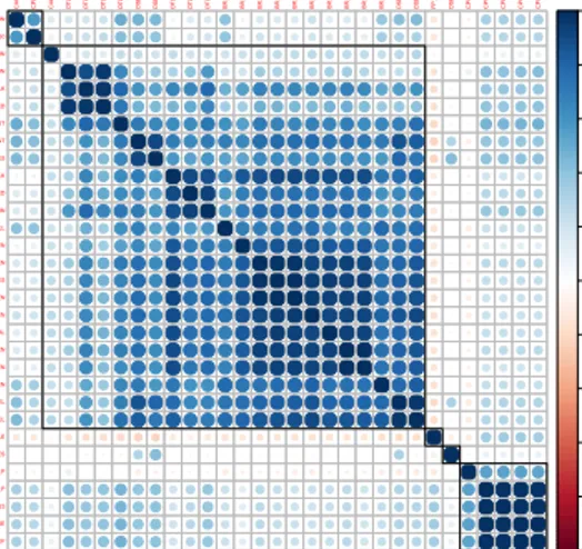
(4) 3.3 Metric-filtering algorithm The filtering step is implemented in the statistical tool R and proceeds as follows: 1. As for the first step, we compute a correlation matrix m of dimension n × n, where entry mij denotes the linear dependence between feature i and j. Set h = h0 2. We classify the features into a small number of disjoint clusters using the k-means algorithm, C = {c1 , c2 , . . . , cr }. All features belonging to a cluster must have a correlation threshold of h. Thus, kmeans is called in a loop fashion to form 1, 2, 3, . . . , n clusters with the initial training set. 3. When a formed cluster has a correlation equal or greater than h among all their features, we found a relevant group: first, we remove all previous representants from the cluster. Then the feature with the highest sum of correlation is determined as representant and stored in a separate list. All group members except the representant are then purged from the matrix. The representant is kept to ensure we are not loosing a feature relevant for forming subsequent clusters. We goto Step 2. If no more clusters can be extracted we goto Step 4. 4. If h > 0.5, we reduce h to h = h · h0 in order to capture less related features and goto Step 2. Otherwise terminate: features that were not grouped so far are also considered as representants. 8 Due to identical start conditions, we assume the counters of repeated runs behave similarly. Based on our results, this assumption seems justified. 9 About four samples per 600 contain overflowing counters.. CPU_CLK_UNHALTED_REF. CPU_CLK_UNHALTED_CORE. CPL_CYCLES_RING123. CPU_CLOCK_UNHALTED_REF_P. CPU_CLOCK_UNHALTED_THREAD_P. DSB_FILL_EXCEED_DSB_LINES. FP_256_PACKED_DOUBLE. DSB_FILL_OTHER_CANCEL. DSB_FILL_ALL_CANCEL. BR_MISP_EXEC_INDIRECT_NEAR_CALL_TAKEN. BR_MISP_EXEC_COND_TAKEN. BR_MISP_EXEC_COND_NON_TAKEN. BR_MISP_RETIRED_CONDITIONAL. BR_MISP_EXEC_INDIRECT_JMP_NON_CALL_RET_TAKEN. BR_MISP_RETIRED_TAKEN. BR_MISP_RETIRED_ALL_BRANCHES. BR_MISP_RETIRED_NOT_TAKEN. BR_MISP_EXEC_RETURN_NEAR_TAKEN. BR_MISP_RETIRED_NEAR_CALL. DTLB_LOAD_MISSES_WALK_DURATION. DTLB_LOAD_MISSES_WALK_COMPLETED. DTLB_LOAD_MISSES_CAUSES_A_WALK. DSB2MITE_SWITCHES_PENALTY_CYCLES. DSB2MITE_SWITCHES_COUNT. DTLB_STORE_MISSES_STLB_HIT. DTLB_STORE_MISSES_WALK_COMPLETED. DTLB_STORE_MISSES_MISS_CAUSES_A_WALK. DTLB_STORE_MISSES_WALK_DURATION. CACHE_LOCK_CYCLES_SPLIT_LOCK_UC_LOCK_DURATION. CPL_CYCLES_RING0. counters, OS statistics and temperature sensors. Since we cannot measure all hardware counters simultaneously, an application is run more than 50 times each time capturing another set of counters. Between the runs of I/O sensitive benchmarks we clear the cache to retain similar start conditions8 . Next, we use Python scripts to merge data, check for consistency and availability of all features, drop overflowing values9 and interpolate the data of the features to the time stamps of the measured power. We derive averaged (node-level) values of features that have been collected at core level. Finally, we build a matrix in which the rows contain samples gathered of each combination of benchmarks and the columns the values of each feature collected. In total, n = 253 features are captured for 78 benchmark runs in the training set and 21 runs in the validation set resulting in a matrix of 112, 303 × 253 (250 MiB CSV file).. M. F. Dolz et al.. CACHE_LOCK_CYCLES_CACHE_LOCK_DURATION. 4. 1. CACHE_LOCK_CYCLES_CACHE_LOCK_DURATION. ●. CPL_CYCLES_RING0. ●. ●. CACHE_LOCK_CYCLES_SPLIT_LOCK_UC_LOCK_DURATION. ●. ●. ●. ●. ●. ●. ●. 0.8. DTLB_STORE_MISSES_WALK_DURATION. ●. DTLB_STORE_MISSES_MISS_CAUSES_A_WALK. ●. ●. DTLB_STORE_MISSES_WALK_COMPLETED. ●. ●. DTLB_STORE_MISSES_STLB_HIT. ●. 0.6 ●. DSB2MITE_SWITCHES_COUNT. ●. DSB2MITE_SWITCHES_PENALTY_CYCLES DTLB_LOAD_MISSES_CAUSES_A_WALK. ●. ●. ●. ●. DTLB_LOAD_MISSES_WALK_COMPLETED. ●. ●. DTLB_LOAD_MISSES_WALK_DURATION. ●. ●. BR_MISP_RETIRED_NEAR_CALL. 0.4. 0.2. ●. ●. ●. BR_MISP_RETIRED_NOT_TAKEN. ●. ●. BR_MISP_RETIRED_ALL_BRANCHES. ●. ●. 0. ●. −0.2. BR_MISP_EXEC_RETURN_NEAR_TAKEN. ●. BR_MISP_RETIRED_TAKEN. ●. BR_MISP_EXEC_INDIRECT_JMP_NON_CALL_RET_TAKEN. ●. BR_MISP_RETIRED_CONDITIONAL. ●. BR_MISP_EXEC_COND_NON_TAKEN. ●. ●. BR_MISP_EXEC_COND_TAKEN. ●. ●. BR_MISP_EXEC_INDIRECT_NEAR_CALL_TAKEN. ●. −0.4. DSB_FILL_ALL_CANCEL DSB_FILL_OTHER_CANCEL. ●. FP_256_PACKED_DOUBLE. ● −0.6. DSB_FILL_EXCEED_DSB_LINES. ●. ●. ●. CPU_CLOCK_UNHALTED_THREAD_P. ●. ●. ●. ●. ●. ●. ●. ●. ●. ●. ●. ●. ●. ●. ●. ●. ●. ●. ●. ●. ●. ●. ●. ●. ●. ●. ●. ●. ●. ●. ●. ●. ●. ●. ●. ●. CPU_CLOCK_UNHALTED_REF_P −0.8. CPL_CYCLES_RING123 CPU_CLK_UNHALTED_CORE CPU_CLK_UNHALTED_REF −1. Fig. 1: Partial correlation matrix obtained from the training set. Blue and red circles stand for positive and negative correlations, respectively. The purpose of the algorithm is to extract a representant for each cluster that is unique to any other feature. As an example, Figure 1 shows a block of a correlation matrix forming 5 clusters. The features of the top left and bottom right are well correlated with each other and behave similar in respect to other features. The big group in the middle contains features showing slightly different behavior in respect to other features.. 3.4 Building reduced models The last step of our methodology is to assemble reduced models, using the subset of representative features obtained in the previous step. The obtained representants are sorted by correlation with respect to the measured power consumption. In order to reduce the number of combinations and derive reduced power models, we set a second threshold f , taking only the f features with the highest correlation to the measured power consumption. This guarantees that only those that are highly correlated with the target of the model will be part of the reduced models. In fact, the linear least-square method delivers good estimations without redundant features but correlated to the estimated variable [17]. In order to estimate the corresponding coefficients, we leverage multiple linear regression. Since there are r representative features, there are r-combinations, i.e., Qr cT = s=1 #cs of representative counters. However, taking into account that in this specific architecture there are only 4 PMC and 3 FIXC registers that can be.

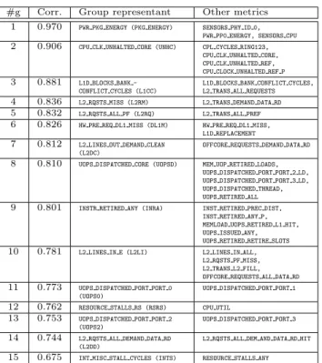
(5) An Analytical Methodology to Derive Power Models based on Hardware and Software Metrics #g. Corr.. Group representant. Other metrics. 1. 0.970. PWR PKG ENERGY (PKG ENERGY). SENSORS PHY ID 0, PWR PP0 ENERGY, SENSORS CPU. 2. 0.906. CPU CLK UNHALTED CORE (UNHC). CPL CPU CPU CPU. 3. 0.881. L1D BLOCKS BANK CONFLICT CYCLES (L1CC). L1D BLOCKS BANK CONFLICT CYCLES, L2 TRANS ALL REQUESTS. 4 5 6. 0.836 0.832 0.826. L2 RQSTS MISS (L2RM). L2 TRANS DEMAND DATA RD. L2 RQSTS ALL PF (L2RQ). L2 TRANS ALL PREF. HW PRE REQ DL1 MISS (DL1M). HW PRE REQ DL1 MISS, L1D REPLACEMENT. 7. 0.812. L2 LINES OUT DEMAND CLEAN (L2DC). OFFCORE REQUESTS DEMAND DATA RD. 8. 0.810. UOPS DISPATCHED CORE (UOPSD). MEM UOP RETIRED LOADS, UOPS DISPATCHED PORT PORT 2 LD, UOPS DISPATCHED PORT PORT 3 LD, UOPS DISPATCHED THREAD, UOPS RETIRED ALL. 9. 0.801. INSTR RETIRED ANY (INRA). INST RETIRED PREC DIST, INST RETIRED ANY P, MEMLOAD UOPS RETIRED L1 HIT, UOPS ISSUED ANY, UOPS RETIRED RETIRE SLOTS. 10. 0.781. L2 LINES IN E (L2LI). L2 LINES IN ALL, L2 RQSTS PF MISS, L2 TRANS L2 FILL, OFFCORE REQUESTS ALL DATA RD. 11. 0.773. UOPS DISPATCHED PORT PORT 0 (UOPS0). UOPS DISPATCHED PORT PORT 1. 12 13. 0.762 0.753. RESOURCE STALLS RS (RSRS). CPU UTIL. UOPS DISPATCHED PORT PORT 2 (UOPS2). UOPS DISPATCHED PORT PORT 3. 14. 0.744. L2 RQSTS ALL DEMAND DATA RD (L2DD). L2 RQSTS ALL DEM AND DATA RD HIT. 15. 0.675. INT MISC STALL CYCLES (INTS). RESOURCE STALLS ANY. CYCLES RING123, CLK UNHALTED CORE, CLK UNHALTED REF, CLOCK UNHALTED REF P. Table 1: List of the 15 most correlated representants in respect to power with h = 0.95 for the correlation threshold between clusters.. read at once, apart from OS statistics and temperature, only combinations of groups of 4 representants are tested. With our methodology, we automatically determined and extracted the top f = 15 representants in respect to the correlation of their group to power consumption. The correlation within a detected group is initialized with h0 = 0.95. The automatically identified representants and the features belonging to their group are given in Table 1.. 5. – Average power. A (bad) prediction for power is the mean value of the power. We expect that any model to be considered valuable should perform better than this naive approach. – Single hardware counters. For example, the RAPL counter PWR PKG ENERGY should provide good estimations for system performance in a linear model. – CPU utilization. Using the utilization statistics of the CPUs, as reported by the OS, should provide fair estimations, CPUs power consumption constitutes more than 50% of the total power consumption on typical systems [1]. – OS statistics. Statistics provided by the OS are comprised of utilization values from the memory subsystem, I/O and network. Since utilization of components is expected to correlate with their contribution to the power consumption, they may give good estimations of the total power consumption. – Temperature sensors. The Poole-Frenkel effect explains how the power-consumption of static leakage power increases with the temperature. It is independent of clockspeed and solely dependent on temperature and voltage [12]. – CPU utilization, OS and sensors. Combinations of previous metrics may improve the predictions.. 4.2 Evaluation of the models. In order to evaluate the reliability of our approach, we compare derived models against the set of basic models. All models are created on the training set and evaluating on the validation data set. Table 2 collects statistics of the prediction accuracy of each model. The Mean and Max columns represent the average and maximum value of the average absolute error, while Q1 and Q3 correspond to the first and third quartiles of the same, respectively. Also root-mean-square error (RMSE) is in4 Validation cluded, it is sensitive to huge absolute errors. The last, To assess the quality and benefit of the models created the coefficient of determination, (R2 ) determines the by our methodology, we employ Quantum Espresso [11], goodness of the fit provided by the model. It is a rough a software suite for ab initio quantum chemistry methestimate for the fraction of points that is explained by ods of electronic-structure calculation and materials mod- the model, thus, an R2 of 1 indicates that the model eling, executing a set of 17 different experiments runexplains all observations, and 0 indicates the opposite. ning on 4 cores of the machine using MPI. Also, our valNote that baseline models are represented from B0 idation set contains the compilation of the Linux kernel to B5, reduced models working solely on hardware counv3.19.2 by executing make -j with 1 to 4 cores. ters range M0 to M5, and combinations of the latter with OS statistics and temperature are represented from D0 to D9 on the table. Also, since there is a large number of combinations among the selected features 4.1 Basic models due to our methodology and also the number of hardware counters that could be read at once, we selected In order to assess the obtained models, we used a set of the most interesting models under those conditions. a simple baseline models:.

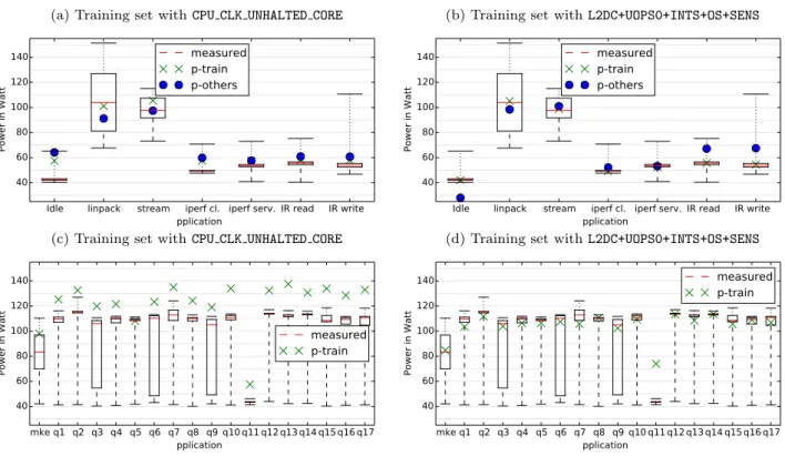
(6) 6. M. F. Dolz et al. R2. #m. Model. Q1. Mean. Q3. Max. RMSE. B0 B1 B2 B3 B4 B5 B6 B7 B8. AVG POWER CPU UTIL OS SENS OS + SENS RAPL PKG POWER CPL CYCLES RING123 CPU CLK UNHALTED CORE MEM UOP RETIRED LOADS. 20.5 11.3 27.9 9.0 5.5 1.4 14.4 14.2 8.6. 24.4 13.6 31.3 11.4 7.5 4.8 19.2 19.0 16.8. 27.3 17.1 34.4 13.3 12.7 6.4 24.6 24.5 25.2. 46.7 59.7 90.5 86.9 88.2 51.6 98.1 98.1 99.2. 24.3 15.1 31.2 17.9 16.6 6.0 22.2 20.6 21.0. 0.00 0.61 0.88 0.97 0.98 0.96 0.89 0.89 0.74. M0 M1 M2 M3 M4 M5. PKG ENERGY + L2DC + UOPS + INTS PKG ENERGY + L2DC + UNHC + DL1M UNHC + L2RM + L2DC + L2LI UNHC + L1CC + L2RQ + UOPSD L2RQ + RSRS + INTS + UOPS2 INRA + UNHR + UNHC + L2RQ + RSRS + UOPS2 + INTS. 0.7 2.1 2.3 2.1 6.5 9.4. 1.5 4.5 5.0 4.4 15.9 15.2. 2.9 6.8 9.2 10.8 25.0 23.0. 50.8 48.0 77.3 70.7 104.1 88.0. 4.5 6.5 10.0 10.1 20.0 18.5. 0.98 0.98 0.96 0.95 0.95 0.96. D0 D1 D2 D3 D4 D5 D6 D7 D8 D9. L2DC L2DC UNHC UNHC L2RQ L2RQ L2RQ INRA INRA INRA. 1.5 1.6 4.1 1.1 4.1 3.7 2.3 3.6 5.9 2.1. 3.1 3.2 6.3 2.5 8.5 7.9 4.0 7.7 10.8 6.1. 5.5 7.0 9.1 4.9 14.9 12.7 7.8 13.2 16.3 9.1. 70.6 76.0 73.6 79.9 97.4 77.6 81.0 97.1 92.0 84.9. 12.1 12.0 12.0 11.8 13.2 13.8 12.2 12.1 15.8 12.8. 0.98 0.99 0.98 0.99 0.96 0.98 0.99 0.97 0.98 0.99. + + + + + + + + + +. UOPS0 + INTS + SENS UOPS0 + INTS + SENS + OS DL1M + L2DC + SENS DL1M + L2DC + SENS + OS RSRS + UOPS2 + INTS + OS RSRS + UOPS2 + INTS + SENS RSRS + UOPS2 + INTS + SENS + OS UNHR + UNHC + L2RQ + RSRS + UOPS2 + INTS + OS UNHR + UNHC + L2RQ + RSRS + UOPS2 + INTS + SENS UNHR + UNHC + L2RQ + RSRS + UOPS2 + INTS + SENS + OS. Table 2: Absolute error of baseline, simple and combined models against the training and validation sets. As can be seen, the naive baseline model B0, average power, leads to almost 0 R2 , confirming this is a bad estimate. Nevertheless, it achieves a mean error of 24.4 W and RMSE of 24.3 which serve as reference. Improved baseline models (from B1 to B4), based on sensors (SENS) improve the accuracy, while CPU utilization only and the operating system aspects are not able to explain the behavior of the validation set. In fact, the OS behavior which also includes CPU utilization leads to a worse model than B0, which is presumably due to overfitting of the training data. On the other hand, some selected hardware counters working alone (models from B6 to B7) are not enough to mimic power consumption, their R2 ranges from 0.74 to 0.89 yet their mean error is more than 16. The model built on top of the RAPL interface achieves R2 of 0.96 and a mean error of 4.8 W, which is considerable well. Despite the goodness of the RAPL interface, for the sake of portability our models should not always depend on this counter. Finally, models created with our algorithmic methodology that work solely with hardware counters (from M0 to M5) provide a good R2 , ranging from 0.95 to 0.98. They provide similar accuracy than RAPL and if used together can improve the accuracy down to 1.5 W. Although their high accuracy, we learned that complementing them with OS statistics and/or temperature sensors (models from D0 to D9), we may even increase their accuracy. It is important to remark that R2 alone is also not sufficient to assess the model quality, for example, M3 and M4 achieve a similar value but the mean error of the latter is higher.. As complementary information, Figure 2 plots power traces in order to compare the real (green points) and estimated (black points) power consumption using some of the baseline cases, ranging from models that work with only one feature to the most elaborated ones combining hardware counters, OS statistics and temperature sensors. We include some benchmarks (training set) but also cases from the validation set. Even though the model shown in each row is created on our training set, we can see interesting differences in the quality of the different models for predicting even the training set. For example, CPU UTIL alone cannot be fitted well to the power of the experiments. Figure 3 shows statistics for the test set and the predicted average. The training set for this experiment is either our general training set. For the training applications we also include the other set which excludes the particular benchmark but includes all other data. The difference between the prediction accuracy of p-train and p-other is an indicator for the importance of a particular benchmark for building the model with the selected features. It can be seen, for example, that iperf client, IOR read and write are well predicted and do not contribute much to the CPU CLK UNHALTED CORE model. For the L2DC+UOPS0+ INTS+OS+SENS model, both IOR read and write are more important. In either case, the idle run is revealing important behavior that needs to be trained. The model built on CPU CLOCK UNHALTED CORE is not fitting the idle case well, it also overestimates the power of the validation set. As expected this feature alone is not sufficient..

(7) An Analytical Methodology to Derive Power Models based on Hardware and Software Metrics. 7. B1 0.61 13.6 CPU UTIL. B5 0.96 4.8 RAPL PKG POWER. B7 0.89 19.0 CPU CLK UNHALTED CORE. D1 0.99 3.2 L2DC+UOPS0+INTS+ SENS+OS. M0 0.98 1.5 PKG ENERGY+ L2DC+UOPS+INT. M5 0.97 15.2 INRA+UNHR+ UNHC+L2RQ+RSS+ UOPS2+INTS M8 0.98 7.7 INRA+UNHR+ UNH+L2RQ+RSS+ UOPS2+INTS+OS M9 0.99 6.1 INRA+UNHR+UNHC+ L2RQ+RSS+UOPS2+ INTS+OS+SENS. Idle. linpack. stream. iperf client. IOR read. IOR write. make. q11. q16. Fig. 2: Real (green) and estimated (black) power consumption traces of some of the training and validation benchmarks using models from the Table 2. The R2 and average error is given as reference after the model number. Note that the X-axis represents the timeline of samples while the y-axis measures power from 38 to 150 W. (b) Training set with L2DC+UOPS0+INTS+OS+SENS. (a) Training set with CPU CLK UNHALTED CORE. measured p-train p-others. 120 100 80 60 40. 120 100 80 60 40. Idle. linpack. stream. iperf cl. iperf serv. IOR read IOR write Application. Idle. 140. 140. 120. 120. 80. measured p-train. 60 40. linpack. stream. iperf cl. iperf serv. IOR read IOR write Application. (d) Training set with L2DC+UOPS0+INTS+OS+SENS. Power in Watt. Power in Watt. (c) Training set with CPU CLK UNHALTED CORE. 100. measured p-train p-others. 140 Power in Watt. Power in Watt. 140. measured p-train. 100 80 60 40. mke q1 q2 q3 q4 q5 q6 q7 q8 q9 q10 q11 q12q13q14 q15q16 q17 Application. mke q1 q2 q3 q4 q5 q6 q7 q8 q9 q10 q11 q12q13q14 q15q16 q17 Application. Fig. 3: Statistics for the validation sets using the models CPU CLK UNHALTED CORE and L2DC+UOPS0+INTS+OS+SENS..

(8) 8. 5 Concluding remarks We presented an effective methodology to determine hardware and software metrics that are important when building power models. With this, a system administrator could alternatively run a daemon, constantly reading those metrics and estimating power consumption, with negligible overhead on the system. Thus, in practice, these models can eventually replace physical wattmeters that are currently necessary to monitor machines on an HPC platform. Our methodology is comprised of a simple but efficient way to construct derived models. First, a calibration step with a few benchmarks is run in order to stress different components of the architecture. It comprises combinations of benchmarks with variation in number of cores used. Each combination is run for 60 s and continuously repeated to collect all hardware and software metrics available on the system. Additionally, we employ the R statistical tool to process all data in order to automatically apply our filtering algorithm. Finally, we manually combine a number of representants that can be accessed at once on our test system to derive our reduced model. Our model is architecture dependent, so the methodology and the models generated should be derived at platform level, however, the methodology can be applied on other architectures. The results demonstrate that the automatically derived models are accurate. It can be observed, that by selecting the most appropriate hardware counters, the goodness of the fit measured in terms of R2 ranges from 0.96 to 0.99, with a mean error down to 3 W without using RAPL counters. By adding OS statistics and especially temperature sensors to the model, the accuracy can be increased potentially. On the contrary, simple models based on temperature and/or OS statistics can yet provide fairly acceptable estimations. In the future, we aim to i) Integrate features for DVFS and multi-socket machines to the model, ii) Develop a kernel module that can provide the estimated power in the proc interface, iii) Automate the tool and provide it as a free and portable package. Acknowledgements This work was supported by the EU Project FP7 318793 “EXA2GREEN” and the German Helmholtz Association’s LSDMA project. We would like to thank Dr. Julen Larrucea, from DKRZ GmbH, for his technical support in configuring the Quantum Espresso software.. References 1. Ashby, S., et al: The opportunities and challenges of Exascale computing. Summary Report of the Advanced Scientific Computing Advisory Committee (ASCAC) Subcommittee (2010). M. F. Dolz et al. 2. Barreda, M., Barrachina, S., Catalán, S., Dolz, M.F., Fabregat, G., Mayo, R., Quintana, E.S.: A framework for power-performance analysis of parallel scientific applications. In: Third Int. Conference on Smart Grids, Green Communications and IT Energy-aware Technologies – Energy 2013 (2013) 3. Barreda, M., Cataln, S., Dolz, M.F., Mayo, R., QuintanaOrtı́, E.S.: Automatic detection of power bottlenecks in parallel scientific applications. Computer Science - Research and Development 29(3-4) (2014) 4. Bellosa, F.: The benefits of event: Driven energy accounting in power-sensitive systems. In: Proceedings of the 9th Workshop on ACM SIGOPS European Workshop: Beyond the PC: New Challenges for the Operating System, pp. 37–42. ACM (2000) 5. Bertran, R., Gonzalez, M., Martorell, X., Navarro, N., Ayguade, E.: Decomposable and responsive power models for multicore processors using performance counters. In: Proceedings of the 24th ACM International Conference on Supercomputing, pp. 147–158. ACM (2010) 6. Castaño, M., Catalán, S., Mayo, R., Quintana-Ortı́, E.: Reducing the cost of power monitoring with dc wattmeters. Computer Science - Research and Development (2014) 7. Cupertino, L., Da Costa, G., Pierson, J.M.: Towards a generic power estimator. Computer Science - Research and Development pp. 1–9 (2014) 8. David, H., Gorbatov, E., Hanebutte, U., Khanna, R., Le, C.: RAPL: memory power estimation and capping. In: 2010 ACM/IEEE International Symposium on LowPower Electronics and Design (ISLPED) (2010) 9. Economou, D., Rivoire, S., Kozyrakis, C., Ranganathan, P.: Full-system power analysis and modeling for server environments. In: Workshop on Modeling Benchmarking and Simulation (MOBS), pp. 13–23 (2006) 10. Ge, R., Feng, X., Song, S., Chang, H.C., Li, D., Cameron, K.W.: Powerpack: Energy profiling and analysis of highperformance systems and applications. IEEE Trans. Parallel Distrib. Syst. 21(5), 658–671 (2010) 11. Giannozzi, P., et al.: Quantum espresso: a modular and open-source software project for quantum simulations of materials. Journal of Physics: Condensed Matter (2009) 12. The Effect of Temperature on Power-Consumption with the Intel i7-2600K. URL http://forums.anandtech.com/ showthread.php?p=32451313 13. Kadayif, I., Chinoda, T., Kandemir, M., Vijaykirsnan, N., Irwin, M.J., Sivasubramaniam, A.: vec: Virtual energy counters. In: Proceedings of the 2001 ACM SIGPLANSIGSOFT Workshop on Program Analysis for Software Tools and Engineering, pp. 28–31. ACM (2001) 14. Kim, H., Vijaykrishnan, N., Kandemir, M., Irwin, M.: Multiple access caches: Energy implications. In: VLSI, 2000. Proceedings. IEEE Computer Society Workshop on, pp. 53–58 (2000) 15. Minartz, T., Kunkel, J., Ludwig, T.: Simulation of power consumption of energy efficient cluster hardware. Computer Science - Research and Development (2010) 16. Mucci, P.J., Browne, S., Deane, C., Ho, G.: Papi: A portable interface to hardware performance counters. In: Proceedings of the Department of Defense HPCMP Users Group Conference, pp. 7–10 (1999) 17. Neter, J., Kutner, M.H., Nachtsheim, C.J., Wasserman, W.: Applied Linear Statistical Models. Irwin (1996) 18. Rivoire, S., Ranganathan, P., Kozyrakis, C.: A comparison of high-level full-system power models. In: Proceedings of the 2008 Conference on Power Aware Computing and Systems, pp. 3–3. USENIX Association (2008).

(9)