A new type of tuned liquid damper and its effectiveness in enhancing seismic performance : numerical characterization, experimental validation, parametric analysis and life cycle based design

Texto completo

(1)PONTIFICIA UNIVERSIDAD CATOLICA DE CHILE ESCUELA DE INGENIERIA. A NEW TYPE OF TUNED LIQUID DAMPER AND ITS EFFECTIVENESS IN ENHANCING SEISMIC PERFORMANCE; NUMERICAL CHARACTERIZATION, EXPERIMENTAL VALIDATION, PARAMETRIC ANALYSIS AND LIFE-CYCLE BASED DESIGN. RAFAEL O. RUIZ. Thesis submitted to the Office of Research and Graduate Studies in partial fulfillment of the requirements for the Degree of Doctor in Engineering Sciences. Advisors: DIEGO LÓPEZ-GARCÍA ALEXANDROS TAFLANIDIS Santiago de Chile, (August, 2015)  2015, Rafael Ruiz.

(2) PONTIFICIA UNIVERSIDAD CATOLICA DE CHILE ESCUELA DE INGENIERIA. A NEW TYPE OF TUNED LIQUID DAMPER AND ITS EFFECTIVENESS IN ENHANCING SEISMIC PERFORMANCE; NUMERICAL CHARACTERIZATION, EXPERIMENTAL VALIDATION, PARAMETRIC ANALYSIS AND LIFE-CYCLE BASED DESIGN. RAFAEL O. RUIZ. Members of the Committee: PROFESOR DIEGO LÓPEZ-GARCÍA PROFESOR ALEXANDROS TAFLANIDIS PROFESOR JOSÉ LUIS ALMAZÁN PROFESOR DIEGO CELENTANO PROFESOR TRACY KIJEWSKI-CORREA PROFESOR GEORGE MAVROEIDIS PROFESOR CRISTIÁN VIAL Thesis submitted to the Office of Research and Graduate Studies in partial fulfillment of the requirements for the Degree of Doctor in Engineering Sciences Santiago de Chile, (August, 2015).

(3) ACKNOWLEDGEMENTS. I would like to thank my supervisors, Dr. Alexandros Taflanidis and Dr. Diego Lopez-Garcia for their technical guidance through my doctoral studies. I have no words to express the important role that you played in my personal and professional life. To the staff at Pontificia Universidad Catolica de Chile and at University of Notre Dame, your support was vital for conducting this dual PhD program. I would like also to express my appreciation to the members of my workgroup, especially to Jose Ignacio Colombo, Juan Carlos Obando, Ioannis Gidaris, Gaofeng Jia, Christopher Vetter and Juan Camilo Medina. Special thanks goes to Christopher Vetter for his help in developing the hazard-compatible stochastic ground motion model that is used for describing seismic risk for the Chilean region and VBM Ingenieria Estructural for provide the dynamic properties of the structure used in Chapter 6. Finally, thank you to Vicerrectoria de Investigacion at Pontificia Universidad Catolica de Chile and to Ministerio de Educacion Superior de Chile for supporting this research and the dual PhD program..

(4) Rafael Ruiz. A NEW TYPE OF TUNED LIQUID DAMPER AND ITS EFFECTIVENESS IN ENHANCING SEISMIC PERFORMANCE: NUMERICAL CHARACTERIZATION, EXPERIMENTAL VALIDATION, PARAMETRIC ANALYSIS AND LIFE-CYCLE BASED DESIGN. Abstract by Rafael Ruiz In the last decades the use of seismic protection devices in Chilean buildings has gained popularity for reducing earthquake losses. Mass dampers (also referenced as inertia dampers), with the most popular representative being the Tuned Mass Damper (TMD), are a potential device for facilitating these tasks; they consist of a secondary mass attached to the primary structure through an equivalent spring and dashpot. Through proper tuning of frequency/damping characteristics, the movement of this secondary mass counteracts the vibration of the primary mass (structure) providing the desired energy dissipation for this vibration. Among the general class of mass damper devices, Tuned Liquid Dampers (TLDs), which consist of a tank filled with some liquid (typically water) whose sloshing within the tank provides the mass damper effect, have some attractive characteristics such as low cost, easy installation and tuning, bidirectional control capabilities and alternative use of the secondary mass (liquid in this.

(5) Rafael Ruiz case). Their popularity, though, has been hindered by the facts that (i) their dynamic behavior is highly non-linear due to wave breaking and (ii) their inherent damping is usual lower than the optimal one, requiring the introduction of submerged elements (to increase this damping) that make the overall behavior even more complex. Other type of liquid dampers that share some of the TLD advantages, the liquid column dampers, offer a simpler modeling but their dynamic behavior is still non-linear since their damping ends up being amplitude dependent, whereas they are strictly restricted to one-directional applications. Additionally, the advantages of any such type of mass dampers particularly for seismic applications in the Chilean region have not been clearly demonstrated; this pertains to both their efficiency, acting as an inertia device, to allow significant energy dissipation for the ground motions common in the region but more importantly to an explicit discussion of the life-cycle cost improvement they can facilitate. The research presented here introduces a new type of liquid mass damper, called Tuned Liquid Damper with Floating Roof (TLD-FR) which combines the favorable characteristics of both TLDs and liquid column dampers, and further examines its efficiency for seismic applications for Chile. The TLD-FR consists of a traditional TLD (liquid tank filled with liquid) with the addition of a floating roof. The sloshing of the liquid within the tank is what still provides the inertia damper effect, but the roof prevents wave breaking phenomena and introduces a practically linear response and a dynamic behavior in a dominant only mode. This creates a vibratory behavior that resembles other types of a linear mass dampers and a framework is developed to.

(6) Rafael Ruiz characterize this behavior with a simple parametric description that can facilitate an easy comparison to such dampers. Within this framework, focus is given on a theoretical/computational characterization of the new device, coupled with an experimental validation of its capabilities and of the established numerical tools. To support these advances an efficient computational approach is formulated to describe the dynamic behavior of liquid tanks and is then extended to describe the behavior of the TLD-FR (address the inclusion of the roof). The aforementioned parametric formulation is then used to develop an approach that facilitates a direct design in the parametric space, as well as an efficient mapping back to the different tank geometries that correspond to each parametric configuration. During this process the efficiency of mass dampers for seismic applications in Chile is also examined by comparing the performance across different types of ground motions, representing different regions around the world. Finally, a versatile life-cycle assessment and design of the new device is established considering risk characterizations appropriate for the Chilean region, so that the cost-benefits from its adoption can be directly investigated. This involves the development of a multi-criteria design approach that considers the performance over the two desired goals: (i) reduction of the total life-cycle cost considering the upfront damper cost as well as seismic losses and (ii) reduction of the consequences, expressed through the repair cost, for low likelihood but high impact events. Through this approach the financial viability of the TLD-FR (competitiveness against TMDs) for enhancing seismic performance is demonstrated..

(7) CONTENTS. Contents ............................................................................................................................... v Figures ............................................................................................................................... viii Tables ................................................................................................................................. xv Chapter 1: Introduction ...................................................................................................... 1 1.1 Motivation......................................................................................................... 1 1.2 Mass Dampers and the Tuned Mass Damper (TMD)........................................ 2 1.3 Special Mass Damper Case: Liquid Dampers .................................................... 9 1.4 Objectives........................................................................................................ 12 Chapter 2: Review of Common Mass Damper Equations of Motion, Description of Typical Tank Geometries of TLDs and Demonstration of Effectiveness for Seismic Protection Against Chilean Earthquakes ................................................................. 16 2.1 Equation of Motion of TMDs, TLCDs and LCVAs ............................................. 16 2.2 Performance and Design Trends for TMDs, TLCDs and LCVAs ....................... 21 2.3 Tank Geometries Used for TLD and TLD-FR .................................................... 25 2.4 Effectiveness of TMDs to suppress earthquakes-induced vibrations for common earthquakes for the Chilean region ........................................... 28 Chapter 3: Efficient Dynamic Analisys of Liquid Storage Tanks ....................................... 39 3.1 Review and Motivation ................................................................................... 39 3.2 Development of the Simplified Sloshing Model (SSM) ................................... 43 3.2.1 Laplace Equation Modification ........................................................ 46 3.2.2 Bernoulli Equation Modification ...................................................... 48 3.2.3 Pressure on the tank walls ............................................................... 50 3.2.4 Summary of the Numerical Approach ............................................. 52 3.3 Validation/Implementation of the Model ...................................................... 55 3.3.1 Tanks Resting on the Ground........................................................... 55 3.4 Summary ......................................................................................................... 79 Chapter 4: Introduction of Tuned Liquid Damper with Floating Roof; Numerical Model Formulation, Experimental Validation and Fundamental Vibration Behavior Exploration .............................................................................................................. 81 v.

(8) 4.1 Introduction of the TLD-FR ............................................................................. 81 4.2 Mathematical Modeling.................................................................................. 83 4.2.1 Inclusion of the floating roof ........................................................... 84 4.2.2 TLD-FR Numerical Model ................................................................. 86 4.3 Experimental Validation.................................................................................. 88 4.3.1 Experimental Setup .......................................................................... 88 4.3.3 Harmonic Response ......................................................................... 93 4.3.4 Seismic Response ........................................................................... 100 4.4 Fundamental Vibration Behavior of TLD-FR and Impact of Floating Roof ... 103 4.5 Summary and General Considerations ......................................................... 108 Chapter 5: Parametric Formulation for TLD-FR Vibration and Design Procedure.......... 110 5.1 Simplification of Equations of Motion through Parametric Formulation..... 111 5.2 Relationship of Transversal Geometry of the Tank to Vibratory Characteristics......................................................................................... 116 5.2.1 Case 1: Rectangular Tanks ............................................................. 117 5.2.2 Case 2: Non-Rectangular Tanks ..................................................... 119 5.3 Design of TLD-FR and Relationships between Parametric Description and Tank Configuration.................................................................................. 124 5.3.1 Selection of Tank Geometry Based on Efficiency Index and Frequency ................................................................................... 125 5.3.2 Damper Configuration ................................................................... 128 5.4 Case Study for Design of TLD-FR ................................................................... 129 5.4.1 Equation of Motion and Response under Stationary Excitation ... 130 5.4.2 Design Procedure ........................................................................... 133 5.4.3 Illustrative Implementation ........................................................... 134 5.5 Summary ....................................................................................................... 141 Chapter 6: Life-Cycle Based Design of TLD-FR Adopting a Seismic Risk Characterization Appropriate for Chile............................................................................................. 144 6.1 Equation of Motion for Multistory Buildings Equipped with TLD-FR ........... 147 6.2 Seismic Risk Quantification and Assessment ................................................ 149 6.2.1 Seismic Risk Quantification ............................................................ 149 6.2.2 Total life-cycle Cost ........................................................................ 152 6.2.3 Repair cost threshold with specific occurrence rate ..................... 155 6.2.4 Simulation-based Risk Assessment ................................................ 156 6.3 Seismic Hazard Modeling .............................................................................. 159 6.4 Design Optimization...................................................................................... 166 6.5 Case Study ..................................................................................................... 169 6.5.1 Seismic Hazard ............................................................................... 169 6.5.2 Structural and Loss Evaluation Models.......................................... 171 6.5.4 Details for Optimization and Validation of Pareto Front ............... 175 6.5.5 Results and Discussion ................................................................... 178 vi.

(9) 6.6 Summary ....................................................................................................... 196 Chapter 7: Conclusions and Future Work ....................................................................... 199 7.1 Summary of Completed Work ...................................................................... 199 7.1.1 Development of an Efficient Computational Procedure to Describe the Dynamic Behavior of Liquid Storage Tanks (Objective 1) .... 201 7.1.2 Numerical Model for TLD-FR, Experimental Validation and Examination of Fundamental Vibratory Characteristics (Objectives 2 and 3) ....................................................................................... 202 7.1.3 Parametric Formulation of TLD-FR Vibration and Design Procedure (Objective 4 and 5) ...................................................................... 204 7.1.4 Life-cycle Analysis of mass dampers for Chilean buildings (Objective 6) ................................................................................................. 206 7.2 Future work ................................................................................................... 208 Appendix A: Eigenvalue Problem Associated with SSM ................................................. 210 Appendix B: Additional Experimental Results ................................................................ 211 Appendix C: Kriging Metamodeling ................................................................................ 216 Appendix D: Review of Stochastic Ground Motion Model used in this Study ............... 218 Bibliography .................................................................................................................... 223. vii.

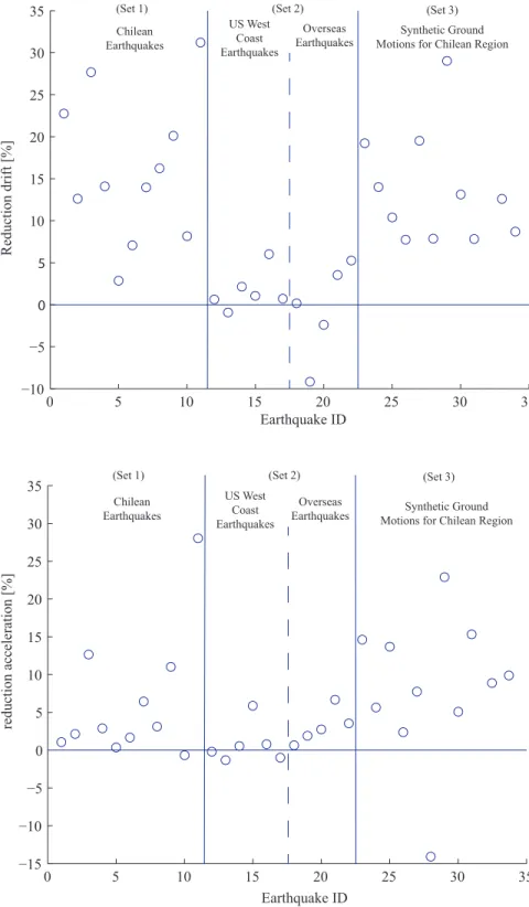
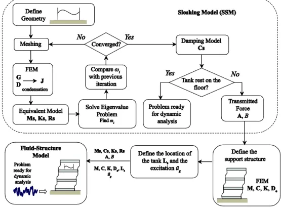
(10) FIGURES. Figure 2.1 TMD (left) and LCVA (right) installed on a single degree of freedom oscillator17 Figure 2.2 Maximum amplification factor for a SDOF equipped with a TMD as a function of TMD characteristics ξd and α for mass ratio of 1%. Damping ratio for SDOF is 2%.......................................................................................................................... 25 Figure 2.3 Scheme of a rectangular tank .......................................................................... 26 Figure 2.4 Description of four different non-rectangular tank geometries, termed as Wtype, V-type, U-type and T-type tanks .................................................................. 27 Figure 2.5 Mass damper efficiency (maximum inter-story drift and acceleration reduction) for 9-story building under different ground motions ........................ 33 Figure 2.6 Comparison of the acceleration of the 9th floor of the building with the response of the TMD in terms of the rms values using a 3s window. Results for four different excitations are reported (characterized through the ID numbers) 36 Figure 2.7 Time-histories for the acceleration of the 9th floor of the building and the displacement of the TMD. Results for four different excitations are reported (characterized through the ID numbers) .............................................................. 37 Figure 3.1 Schematic for liquid storage tank with arbitrary geometry. Various boundaries utilized in the SSM also shown. ............................................................................ 43 Figure 3.2 Procedure for SSM (top) and its use in fluid-structure interaction problems (bottom).Illustrative excitation in the latter case for structure corresponds to acceleration at its base. ........................................................................................ 54 Figure 3.3 Fundamental sloshing period of rectangular tanks as a function of length L and aspect ratio R. Comparison between the SSM, Housner model and analytic solution of (Chen et al. 1996) is shown. ............................................................... 59 Figure 3.4 Second sloshing period of rectangular tanks as a function of length L and aspect ratio R. Comparison between the SSM and analytic solution of (Chen et al. 1996) is shown. ..................................................................................................... 60 viii.

(11) Figure 3.5 Third sloshing period of rectangular tanks as a function of length L and aspect ratio R. Comparison between the SSM and analytic solution of (Chen et al. 1996) is shown. ..................................................................................................... 60 Figure 3.6 Normalized transmitted force to the walls of a rectangular tank, with L=9.144m for different values of R under harmonic response for different period ratios rsp (excitation period to fundamental sloshing period) .............................. 63 Figure 3.7 Sloshing period as a function of a and h for W- and U-type tanks. Cases correspond to L=380mm and H=76mm ............................................................... 68 Figure 3.8 Seismic response histories (expressed through the transmitted force to the base) of non-rectangular tanks A and B under El Centro excitation .................... 70 Figure 3.9 Displacement response of the 9-floor building with a rectangular TLD under seismic excitation .................................................................................................. 74 Figure 3.10 Acceleration response of the 9-floor building with a rectangular TLD under seismic excitation .................................................................................................. 75 Figure 3.11 Displacement response of the 9-floor building with a U-type TLD under seismic excitation .................................................................................................. 77 Figure 3.12 Acceleration response of the 9-floor building with a U-type TLD under seismic excitation .................................................................................................. 78 Figure 4.1 Schematic for a rectangular TLD-FR................................................................. 82 Figure 4.2 Scheme of the coincident mesh between liquid and floating roof and illustration example for derivation of damping matrix ........................................ 85 Figure 4.3 Scheme for experimental setup for validation of the TLD-FR ......................... 89 Figure 4.4 Normalized transmitted force (non-dimensional) for experimental configurations without external damping under harmonic excitation for different excitation periods. (i) Numerical and (ii) experimental results under different excitation amplitudes are compared .................................................................... 95 Figure 4.5 Floating roof amplitude (normalized by excitation amplitude) for experimental configurations without external damping under harmonic excitation for different excitation periods. (i) Numerical and (ii) experimental results under different excitation amplitudes are compared .............................. 96 Figure 4.6 Normalized transmitted force (non-dimensional) for experimental configurations with external damping under harmonic excitation for different ix.

(12) excitation periods. (i) Numerical and (ii) experimental results under different excitation amplitudes are compared .................................................................... 97 Figure 4.7 Floating roof amplitude (normalized by excitation amplitude) for experimental configurations with external damping under harmonic excitation for different excitation periods. (i) Numerical and (ii) experimental results under different excitation amplitudes are compared..................................................... 98 Figure 4.8 Ground motion imposed as excitation, corresponding to the ground motion recorded at Melipilla station during the 1985 Chile earthquake ....................... 100 Figure 4.9 Transmitted force for tanks A and B under seismic excitation. Comparison between numerical and experimental results shown. ....................................... 101 Figure 4.10 Floating roof amplitude for tanks A and B under seismic excitation. Comparison between numerical and experimental results shown.................... 102 Figure 4.11 Photograph sequence of a TLD-FR (upper row) and TLD (lower row) under seismic excitation. Same tank geometry used in the two cases. Wave breaking and nonlinear behavior is evident in the latter but the presence of the floating roof keeps former practically linear. .................................................................. 103 Figure 4.12 Modal shapes for a tank with R=0.5, L=8m. For TLD-FR the beam stiffness is set to EI=1400Nm2 ............................................................................................. 105 Figure 4.13 Transfer function for TLD and TLD-FR employing a floating roof with a EI=1400Nm2. Different tank geometries examined. .......................................... 106 Figure 4.14 Transfer function for TLD and TLD-FR employing a floating roof with a EI=1400000Nm2. Different tank geometries examined..................................... 107 Figure 4.15 Results for non-symmetric tank for TLD and TLD-FR (a) Schematic of a tank and its geometric details, (b) mode shapes for first and second mode and (c) frequency response function. Value of EI is 1400000Nm2 for the TLD-FR. ....... 108 Figure 5.1 Fundamental periods and efficiency indexes for different TLD-FR for rectangular tanks ................................................................................................ 118 Figure 5.2 Comparison of efficiency indexes for different TLDs-FR and TLDs for different rectangular tanks ................................................................................................ 119 Figure 5.3 Iso-curves for fundamental periods and efficiency indexes of a TLD-FR employing a U-tank. Upper row corresponds to: (a) R=0.2 and L=4m, center row to (b) R=0.2 and L=6m and lower row to (c) R=0.4 and L=4m .......................... 121 x.

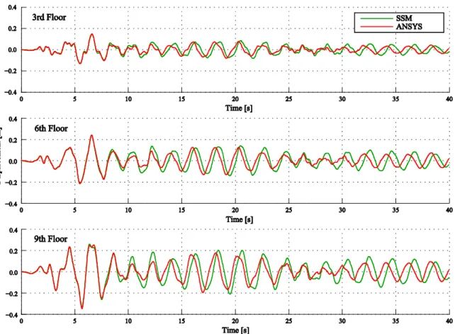
(13) Figure 5.4 Iso-curves for fundamental periods and efficiency indexes of a TLD-FR employing a T-tank. Upper row corresponds to: (a) R=0.2 and L=4m, center row to (b) R=0.2 and L=6m and lower row to (c) R=0.4 and L=4m .......................... 122 Figure 5.5 Optimal frequency and damping ratio for different efficiency indexes and mass ratios for a TLD-FR attached to a SDOF under stationary seismic excitation. Stationary variance is utilized as objective function. ......................................... 136 Figure 5.6 Responses of the structure (as percentage reduction over the uncontrolled response) and of the floating roof under optimal design for a TLD-FR attached to a SDOF under stationary seismic excitation. Stationary variance is utilized as objective function for calculating the optimal damper design configuration.... 137 Figure 5.7 Characteristics for the different tank geometries that match with the optimal values of the TLD-FR and satisfy the various chosen constraints for the roof displacement. The value Rm/mm is also shown. Value of R is used as reference for the comparisons and is included in all the subplots. With respect to the constraints for the floating roof, the configurations are separated into three different groups satisfying the different constraints (denoted with different symbols) .............................................................................................................. 139 Figure 6.1 Modeling approach for seismic risk quantification ....................................... 150 Figure 6.2 Seismic hazard map for Chile from USGS (peak ground acceleration with probability of being exceeded 10% in 50 years) [available at http://earthquake.usgs.gov/earthquakes/world/chile/gshap.php] .................. 161 Figure 6.3 Illustration of hazard-compatible ground motion modeling for Chilean GMPEs; comparison of GMPE and model predictions for different M − rrup values for peak ground acceleration (left) and peak spectral acceleration Spa for 5% damped elastic SDOFs with period Tsd 2 s (right) ............................................... 164 Figure 6.4 Illustration of hazard-compatible ground motion modeling for Chilean GMPEs; for different characteristic M − rrup values spectral plots for peak acceleration of 5% damped elastic SDOFs (comparison between GMPE and model shown) as well as sample ground motions created by the model .......... 165 Figure 6.5 Arias intensity (left) and significant duration (right) as a function of M − rrup for the established ground motion model (surface plots) as well as samples from regional (for Chile) recorded ground motions .................................................... 166 Figure 6.6 Probability of exceedance of different thresholds for peak ground acceleration PGA and spectral acceleration Spa of a 5% damped elastic SDOF with period Tsd 2 s. ............................................................................................. 171 xi.

(14) Figure 6.7. Comparison between the estimated performance through the kriging metamodel and the high-fidelity model for the Pareto optimal solutions for design case corresponding to value of γ=0.7 and upfront cost assumption of 1700 $/ton ................................................................................................................... 177 Figure 6.8 Pareto front for the total life-cycle cost C and repair cost threshold with probability of exceedance 10% in 50 years, Cthresh, for different efficiency indexes and different assumptions for upfront damper cost (blue is low damper cost, red is medium and black is high). Results correspond to probabilistic structure. Mass ratio under optimal design and decomposition of total cost to upfront cost and life-cycle repair cost is also shown in parenthesis.............................................. 180 Figure 6.9 Pareto front for the total life-cycle cost C and repair cost threshold with probability of exceedance 10% in 50 years, Cthresh, for different efficiency indexes and different assumptions for upfront damper cost (blue is low damper cost, red is medium and black is high). Results correspond to nominal structure. Mass ratio under optimal design and decomposition of total cost to upfront cost and life-cycle repair cost is also shown in parenthesis.............................................. 181 Figure 6.10. Pareto front for the total life-cycle cost C and repair cost threshold with probability of exceedance 10% in 50 years, Cthresh, for different efficiency indexes and and an upfront damper cost of 1000$/ton. Results for both the nominal structure and probabilistic structure are shown. ............................................... 182 Figure 6.11. Variation of mass ratio r corresponding to optimal solution against the total life-cycle cost C across the Pareto front for different efficiency indexes and different assumptions for upfront damper cost (blue is low damper cost, red is medium and black is high). Results correspond to probabilistic structure. ....... 184 Figure 6.12. Variation of mass ratio r corresponding to optimal solution against the total life-cycle cost C across the Pareto front for different efficiency indexes and different assumptions for upfront damper cost (blue is low damper cost, red is medium and black is high). Results correspond to nominal structure ............... 185 Figure 6.13. Variation of mass ratio r corresponding to optimal solution against repair cost threshold with probability of exceedance 10% in 50 years Cthresh across the Pareto front for different efficiency indexes and different assumptions for upfront damper cost (blue is low damper cost, red is medium and black is high). Results correspond to probabilistic structure. ................................................... 186 Figure 6.14. Variation of mass ratio r corresponding to optimal solution against repair cost threshold with probability of exceedance 10% in 50 years Cthresh across the Pareto front for different efficiency indexes and different assumptions for xii.

(15) upfront damper cost (blue is low damper cost, red is medium and black is high). Results correspond to nominal structure. .......................................................... 187 Figure 6.15. Variation of damping ratio ξm corresponding to optimal solution across the Pareto front against the corresponding optimal mass ratio r for different efficiency indexes and different assumptions for upfront damper cost (blue is low damper cost, red is medium and black is high). Results correspond to probabilistic structure. ........................................................................................ 189 Figure 6.16. Variation of damping ratio ξm corresponding to optimal solution across the Pareto front against the corresponding optimal mass ratio r for different efficiency indexes and different assumptions for upfront damper cost (blue is low damper cost, red is medium and black is high). Results correspond to nominal structure.............................................................................................................. 190 Figure 6.17. Variation of frequency ratio a corresponding to optimal solution across the Pareto front against the corresponding optimal mass ratio r for different efficiency indexes and different assumptions for upfront damper cost (blue is low damper cost, red is medium and black is high). Results correspond to probabilistic structure. ........................................................................................ 191 Figure 6.18. Variation of frequency ratio a corresponding to optimal solution across the Pareto front against the corresponding optimal mass ratio r for different efficiency indexes and different assumptions for upfront damper cost (blue is low damper cost, red is medium and black is high). Results correspond to nominal structure.............................................................................................................. 192 Figure 6.19. Variation of ratio of upfront to total cost against the corresponding optimal repair cost threshold with 10% of probability of exceedance in 50 years Cthresh across the Pareto front of optimal solutions for different efficiency indexes and different assumptions for upfront damper cost (blue is low damper cost, red is medium and black is high). ................................................................................. 193 Figure 6.20. Repair cost decomposition for some representative configurations corresponding to optimal solutions across the Pareto front. Results for structure without damper also shown (unretrofitted structure)....................................... 194 Figure 6.21. Impact of neglecting structural uncertainties in the design stage. Performance (total life-cycle cost C and repair cost threshold with probability of exceedance 10% in 50 years, Cthresh) for different efficiency indexes and different assumptions for upfront damper cost (blue is low damper cost, red is medium and black is high) for the probabilistic structure is shown. Pareto front for this case as well as performance for the optimal solution corresponding to the nominal structure are shown.............................................................................. 195 xiii.

(16) Figure B.1 Free response of the floating roof for configurations identified as Tank A and Tank B obtained after imposing a pulse-like excitation. .................................... 211 Figure B.2 Free response of the floating roof for configurations identified as Tank C and Tank D obtained after imposing a pulse-like excitation. .................................... 212 Figure B.3 Free response of the floating roof for configurations identified as Tank E and Tank F obtained after imposing a pulse-like excitation. ..................................... 212 Figure B.4 Floating roof amplitude for tanks C and D under seismic excitation. Comparison between numerical and experimental results shown.................... 213 Figure B.5 Transmitted force for tanks C and D under seismic excitation. Comparison between numerical and experimental results shown. ....................................... 214 Figure B.6 Floating roof amplitude for tanks E and F under seismic excitation. Comparison between numerical and experimental results shown.................... 214 Figure B.7 Transmitted force for tanks E and F under seismic excitation. Comparison between numerical and experimental results shown. ....................................... 215. xiv.

(17) TABLES. Table 2.1 Characteristics of the chosen Chilean earthquakes .......................................... 31 Table 2.2 Characteristics of earthquakes chosen from other regions of the world ......... 32 Table 2.3 Characteristics of the chosen synthetic ground motions compatible with Chilean hazard....................................................................................................... 32 Table 3.1 Sloshing periods for a rectangular tank with L=9.144m and R=0.5 ................. 58 Table 3.2 Comparison of transmitted force to the ground obtained by different methods for the considered rectangular tanks under different earthquake excitations ... 65 Table 3.3 Details of the tank geometries selected from (Idir et al. 2009) and (Gardarsson 1997) and used here ............................................................................................. 66 Table 3.4 Fundamental sloshing period [in s] for the considered non-rectangular tanks 66 Table 3.5 Peak response values of the 9-floor structure with a rectangular TLD under seismic excitation .................................................................................................. 75 Table 3.6 Peak response values of values of the 9-floor structure with a U-type TLD under seismic excitation ....................................................................................... 78 Table 4.1 Details of the TLD-FR configurations considered in the experimental study ... 90 Table 4.2 Undamped sloshing periods of the TLD-FR configurations considered in the experimental study ............................................................................................... 92 Table 4.3 Experimental damping ratios for the different TLD-FR configurations ............ 92 Table 6.1 Characteristic of the cost estimation. Values for fragility curves related to partitions, contents and acoustical ceiling ......................................................... 174 Table D.1 Optimized coefficients for the predictive relationships of the stochastic ground motion model parameters to achieve GMPE compatibility ............................... 222. xv.

(18) INTRODUCTION. 1.1 Motivation In modern urban areas there is an increasing trend to build light and flexible structures. In order to enhance the performance of such structures addition of supplemental devices is frequently promoted to control undesirable vibrations due to exposure to dynamic excitations such as winds or earthquakes (Housner et al. 1997; Zemp et al. 2011). Earthquake-induced (short-duration and large amplitude) vibrations may result in significant damages to structural and non-structural components and building-contents. Recent examples of such damages are discussed in Inokuma and Nagayama 2013 or Saatcioglu et al. 2013. Additionally, wind-induced (longer-duration but smaller amplitude) vibrations can also contribute to failure for serviceability limit states (cladding damage, elevator malfunction) as well as to fatigue damage (large number of lower amplitude oscillations) and, to some extreme cases (very strong winds or errors in designs/construction), even to structural failure (Sain and Kishen 2007). To alleviate such impacts, different techniques have been proposed to control natural hazard induced-vibration of structures, with one of the most popular being the. 1.

(19) introduction of passive devices, i.e. devices that require no external power supply. These devices impart forces counteracting directly the motion of the structure. Examples include viscous and viscoelastic dampers, friction dampers, hysteretic dissipaters, base isolation systems or inertial-type of dampers generally referenced as mass dampers (Soong and Dargush 1997; C. Christopoulos and A. Filiatrault 2006; Gutierrez Soto and Adeli 2013). They have prevailed in structural control applications, including in control application in Chile (Zemp et al. 2011; De la Llera et al. 2004), over active devices due to the large power demand of the latter (Housner et al. 1997) that cannot be reliably provided, and the fact that a significant life-cycle cost improvement arguing for the adoption of active devices has never been comprehensively proven. Note, furthermore that some of these passive devices can be extended to operate in semi-active mode by controlling in real-time their characteristics, such as orifice openings for viscous dampers that alter the viscosity coefficient of spring characteristics for TMDs (Housner et al. 1997; Sun et al. 2014).. 1.2 Mass Dampers and the Tuned Mass Damper (TMD) Perhaps the most commonly used passive device are mass dampers (frequently also referenced as inertia dampers), which consist of an inertial element (secondary mass) attached to a higher floor of the structure to be controlled (primary mass). Through appropriate tuning of its vibratory characteristics (meaning typically tuning to a specific mode of vibration for the structure), the secondary mass resonates out-of-phase 2.

(20) with the point of connection to the structure, reducing through its own dynamic response the vibration level of the primary mass (Den Hartog 1985). When that secondary mass corresponds to a single degree of freedom oscillator then the device is known as a Tuned Mass Damper (TMD). An equivalent interpretation of TMDs is that they correspond to mass dampers for which the entire additional mass (of the inertia damper) responds in a single mode and therefore that entire mass ultimately participates in the suppression of the vibration of the primary mass. It is well understood that mass dampers impact the vibratory characteristics only in the range close to their own frequency, meaning that (a) they can suppress only a specific mode and that (b) the aforementioned tuning is very important for their efficiency (Den Hartog 1985; Gutierrez Soto and Adeli 2013; Oberguggenberger and Schmelzer 2014). Implementation of mass dampers may take different forms, for example directly a mass-spring-damper configuration or a swinging pendulum with additional elements to provide a damping effect to its vibration. A more detailed description of such configurations can be found in (Matta and De Stefano 2009; Gutierrez Soto and Adeli 2013). Mass dampers have been proven particularly advantageous for flexible buildings since they are economical and can be relatively easily implemented as an add-on to existing or new structures. Application of multiple mass dampers can be also considered to provide more efficient vibration suppression or even control of different modes of vibrations (Abe and Fujino 1994; Yang et al. 2015; Park and Reed 2001). For example for Taipei 101, which stands 508 m above ground 3.

(21) level in a region which experiences strong winds, earthquakes, and typhoons, three different TMDs have been applied, one of which was, at that point, the largest TMD in the world with mass of 660 tons (Tamboli et al. 2008). The first inertia damper application was actually presented by (Frahm 1911) to reduce hull motion of ships. Today it is commonly used in buildings, automobiles, antennas, and in general very diverse dynamical system where vibration suppression is desired. The modeling of all devices belonging in the mass damper category can be equivalently expressed as single-degree-of-freedom oscillator (Chang 1999) with a specified mass connected to the primary structure though a spring and a dashpot. The difference between the different type of inertia damper devices is how the spring/dashpot configuration is ultimately established with an additional distinction of whether the total mass participates in the vibration suppression (Chang 1999), whereas some exhibit nonlinear vibratory characteristics with respect to the damping (dashpot) properties (Rudinger 2007). Semi-active implementations further differentiate these dampers (Hrovat et al. 1983; Sun and Nagarajaiah 2014; Lin et al. 2015). Such mass dampers have been proposed in the literature for improving the dynamic performance of structures under a variety of dynamic excitations, including seismic excitations, though at this case with a reduced overall effectiveness, an effectiveness which additionally greatly depends on the characteristics of the excitation (Gutierrez Soto and Adeli 2013; Lin et al. 2001). This should be attributed to the fact that earthquakes are short-duration, non-stationary excitations, frequently (in near-fault 4.

(22) regions) with impulsive characteristics (Mavroeidis and Papageorgiou 2003). On the other hand, mass dampers, being inertia devices, require typically some rise-time for their activation (Lin et al. 2010), so that their own vibration becomes large enough to facilitate the desired energy dissipation for the motion of the primary structure. If the characteristics of the ground motion are such that there is not sufficient time for this inertia mode of operation (meaning an impulsive rather than a gradual built-up of the excitation), then the efficiency of the mass dampers is expected to be small. Still, a variety of studies have demonstrated the potential of mass dampers in reducing seismic vibrations (Tributsch and Adam 2012; Hoang et al. 2008; Wong 2008; Miranda 2005). The caveat, though, that the discussion above demonstrates is that one needs to examine careful the characteristics of anticipated regional excitations before promoting such a solution. The design, now, of mass dampers involves an optimization problem in which the spring/dashpot values are selected based on some performance criteria. For the spring this means, as discussed earlier, match to a specific modal frequency of the primary structure (impact to only a specific mode as discussed earlier). In this context, many researchers have addressed the optimal mass damper design under different excitation conditions (Soong and Dargush 1997; Gutierrez Soto and Adeli 2013) while examining different possible performance quantifications or even the implementation of multiple mass dampers (Abe and Fujino 1994).. The most popular approaches. correspond to reducing the response to (a) sinusoidal excitation [objective corresponds 5.

(23) to the maximum value of the amplification factor (Den Hartog 1985)] or (b) white noise excitation [objective corresponds to the area under the squared amplification factor giving the response-variance (Warburton 1982)]. The latter can easily be extended to minimization of the response to stationary excitation with any desired power spectrum (Yalla and Kareem 2000) [objective is related to the area of the squared amplification factor multiplied by the power spectrum of the excitation]. Approaches also exist that have looked at reliability definitions for the performance under stationary excitation, i.e. not just simple statistics such as the response-variance, by solving the so-called firstpassage problem (Taflanidis et al. 2007; Marano et al. 2007). Such procedures are definitely reasonable for wind excitation since the latter can be adequately described as stationary random processes (Simiu and Scanlan 1996). For seismic applications they might be problematic since the excitation does not have stationary characteristics. Still, they are popular even for design against earthquakes (Daniel and Lavan 2014; Moutinho 2012), the underlying assumption being that the strongest part of the ground motion can be described trough a stationary random process (Hoang et al. 2008) or that at least a design within this context will lead to a solution that is not far away from the optimal solution that would be obtained if a more faithful representation of the excitation and the performance of the structure was used. For mass dampers this seems a reasonable assumption since the fundamental requirement for proper design is the matching of its frequency to a modal frequency of the primary mass, which is to some degree independent of the excitation modeling as 6.

(24) has been demonstrated in (Taflanidis 2003) when comparing the design considering harmonic or white noise excitations. This design of course also provides an optimum equivalent dashpot; for this parameter it is well understood that the performance is quite insensitive to values of the dashpot higher than the actual optimum but exhibits very high sensitivity to lower values (Warburton 1982; Taflanidis 2003). This trend can be attributed to an inability to dissipate quickly-enough the vibration of the mass damper with kinetic energy ultimately being transferred back to the primary structure [with extreme case demonstrating beat-phenomenon behavior (Yalla and Kareem 2001)]. As long as lower values of the dashpot coefficient (from this optimal level) are avoided, good performance can be in general accomplished. It should be further stressed that for seismic applications, it is well understood that mass dampers will not necessarily reduce the peak vibration characteristics for all possible transient, seismic excitations, something that widely depends on the characteristics of the excitation itself (Giuliano 2013). Through a proper design, though, some contribution towards reduction of the seismic risk is anticipated (Tributsch and Adam 2012; Hoang et al. 2008; Wong 2008; Miranda 2005). Of course other considerations do exist for mass damper design. An important one is the displacement of the secondary mass itself (secondary design goal), beyond the aforementioned vibration suppression of the primary mass (main design goal). This displacement ultimately imposes requirements of the clearance around the secondary mass to facilitate its vibration amplitude. Approaches have been proposed in the 7.

(25) literature to directly consider this displacement as design goal, typically through a multiobjective setting (Kim and Kang 2012; Chakraborty et al. 2012). Another important consideration is the effect of uncertainties related to properties of the primary structure (damping but more importantly factors affecting modal properties such as mass and stiffness). Poor estimation of the dynamic characteristics of the structure can lead to a significant mistune that translates into a loss of performance (Hoang et al. 2008; Mei et al. 2004; Oberguggenberger and Schmelzer 2014). This has motivated researchers to look into the robust design of mass dampers under excitation and structural uncertainties (Chakraborty and Roy 2011; Debbarma et al. 2010a; Debbarma et al. 2010b; Taflanidis et al. 2007), typically adopting stationary assumptions for the description of the excitation. Despite the aforementioned efforts, limited attention has been given in the lifecycle assessment of the performance of mass dampers under seismic excitation adopting more comprehensive modeling frameworks to describe the excitation and addressing through a more meaningful approach the cost-benefit aspects of mass damper implementation. Larger dampers always provide greater benefits (bigger reduction for the vibration of the primary structure) but evidently have a larger associated cost that needs to be explicitly considered in the design process. Recent work (Lee et al. 2012) addressed the life-cycle benefits of adding TMDs but did not extend this approach to the more challenging aspects of design that requires direct incorporation of considerations about upfront cost. Even though such a framework for life-cycle cost 8.

(26) based design of other type of dissipative devices exist (Taflanidis and Beck 2009), it has never been applied to mass dampers. Furthermore this framework has only considered the design that directly minimizes the life-cycle cost without examining additional criteria such as losses for low likelihood but high impact events, representing more complex attitudes towards risk.. 1.3 Special Mass Damper Case: Liquid Dampers A special case of mass dampers are liquid dampers for which the secondary mass corresponds to a liquid (typically water) inside a (a) tank (Kareem and Sun 1987; Fujino et al. 1988) or a (b) U-shaped tube (Sakai et al. 1989). Implementation (a) is known as Tuned Liquid Damper or Tuned Sloshing Damper (TLD/TSD) and (b) as liquid column damper and has two different representatives the Tuned Liquid Column Damper (TLCD) (Sakai et al. 1989) and the Liquid Column Vibration Absorber (LCVA) (Hitchcock et al. 1997), the distinction between them being whether the U-tube has uniform or not, respectively, cross-section. These liquid dampers have some distinct advantages (A.1) lower installation costs, (A.2) easy tuning process for their fundamental frequency and (A.3) potential alternative use of the secondary mass which for this case is not simply a dead mass for the structure (for example water can be used during fire emergencies). Next each of the aforementioned type of liquid dampers is separately discussed Tuned Liquid Dampers: TLDs have been demonstrated to effectively control vibrations induced by winds (Fujii et al. 1990; Tamura et al. 1995; Kareem 1990) while 9.

(27) also having the potential to mitigate earthquakes-induced vibrations (Banerji et al. 2000; Banerji and Samanta 2011; Zahrai et al. 2012). They consist of a tank filled with liquid (usually water), the sloshing of which counteracts the motion of the structure providing energy dissipation for the vibration of the latter. It is well-understood that not the entire liquid mass participates in this sloshing motion in a specific mode whereas additional challenges exist because of wave-breaking phenomena that impose a non-linear behavior (Sun et al. 1995; Reed et al. 1998). The oscillation characteristics (fundamental frequency) of the liquid are related to the dimensions of the tank and the depth of the liquid (Chen et al. 1996). Beyond the aforementioned advantages (A.1-A.3) TLDs are additionally attractive (over other type of mass dampers) because their bidirectional control capabilities (ability to tune liquid sloshing in both directions through appropriate selection of length). Their dynamic behavior, though, is typically highly nonlinear as explained above due to wave breaking phenomena, and their inherent level of damping (due to drag forces in the vibrating liquid) is typically much less than the level that would lead to an optimal suppression of the vibration of the structure (Soong and Dargush 1997). In other words the optimal equivalent dashpot coefficient cannot be achieved and the lower established damping will lead, as discussed earlier, to a significantly lower performance of the mass damper. While higher levels of damping can be attained by adding submerged obstacles, the resulting behavior is very difficult to model and, consequently, to reliably predict (Kaneko and Ishikawa 1999). It should be also stressed that even though TLDs have been primarily considered and widely 10.

(28) implemented to control wind-induced vibrations, many researchers are currently investigating how to develop practical TLDs than could be used to effectively control seismically induced vibrations. In general, the research efforts related to TLDs in recent years have primarily focused on: (a) developing relatively simple analytical tools to model wave breaking and damping (Tait 2008; Love and Tait 2010; Maravani and Hamed 2011); (b) establishing strategies to provide additional damping without introducing excessively complicated modeling issues (e.g. submerged screen, nets, baffles, etc.) (Modi and Munshi 1998; Modi and Akinturk 2002; Biswal et al. 2003; Kaneko and Ishikawa 1999); and (c) implementing active and semi-active control strategies (Zahrai et al. 2012; Shang and Zhao 2008). Despite the aforementioned advantages and relevant research efforts, the popularity of TLDs has remained relatively low, something that should be attributed to the complexities in modeling both the wave breaking and the non-linearities related to the damping-enhancement elements. These complexities lead to numerical models that are difficult to implement, and to challenging design procedures. Liquid Column Dampers: To address this barrier, liquid column mass dampers, namely the TLCD and the LCVA, have been introduced and given significant attention by various researchers (Chang and Hsu 1998; Sadek et al. 1998; Yalla and Kareem 2000; Won et al. 1997; Balendra et al. 1995; Taflanidis et al. 2007). As discussed before, these devices consist of a U-shaped tube, or, as can be equivalently considered, of two liquid containers interconnected at their lower part with a horizontal tube or pipe such that 11.

(29) the liquid is able to move from one container to the other. The motion of the liquid within the horizontal tube counteracts the motion of the structure and provides energy dissipation, resulting in an effectiveness of the TLCD/LCVA that is directly related to the mass in the tube and not to the overall liquid mass (Chang 1999). This may be equivalently considered as not the entire liquid mass participating in the horizontal mode of vibration. The frequency of oscillation of the liquid is directly related to the length of the liquid column, which is the only parameter that can be adjusted to establish the desired tuning characteristics. The horizontal tube can be also used to place an element (typically a valve or an orifice plate) that provides energy dissipation (damping) (Sakai et al. 1989), and the damping level can potentially be controlled in a passive or semi-active way (Yalla and Kareem 2003). The vibration of the liquid within the tube prevents any wave-breaking phenomena, thus leading to simpler models (single degree of freedom behavior) than those of TLDs. However, TLCD/LCVA devices are restricted to one-directional applications (Samali 1990), and their behavior is still nonlinear because damping is amplitude-dependent due to the presence of the orifice (Taflanidis et al. 2007).. 1.4 Objectives Motivated by the aforementioned limitations of TLDs and liquid column dampers but also the advantages that liquid mass dampers have to offer, the objective of this research is to propose a modification of the traditional TLD through a simple 12.

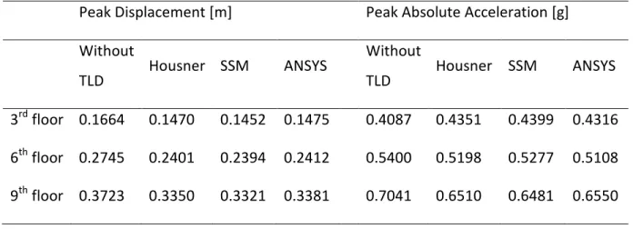
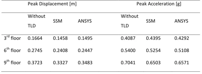
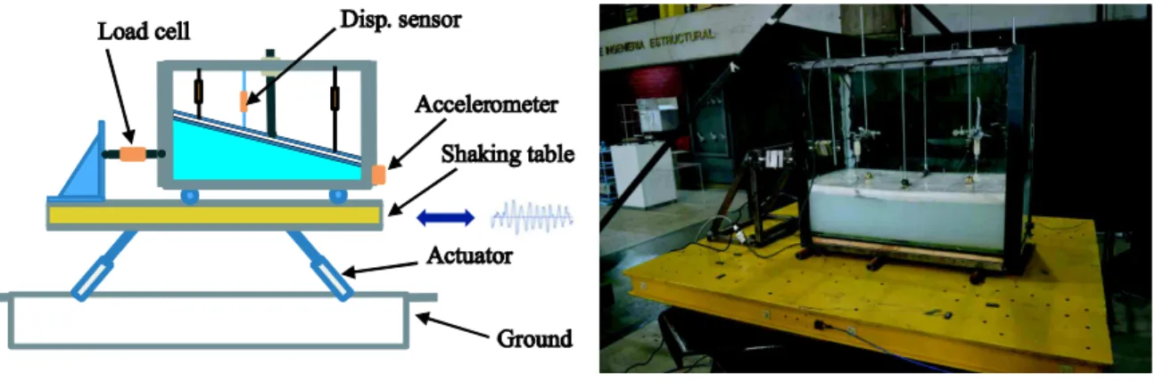
(30) introduction of a floating roof that addresses the aforementioned challenges that have restricted its popularity. This new device is termed TLD with floating roof (TLD-FR). Another objective is to establish a simplified framework for easy comparison of the new device to TLDs as well as TMDs. These goals include both a theoretical and experimental component, while they also involve the development of new numerical tools to facilitate a computationally simpler description of the behavior of TLDs. Additionally, the efficiency of mass dampers for seismic protection in the Chilean region is examined in detail and a life-cycle design of the new device (or as it will be demonstrated later generally of mass dampers) is developed that (a) provides a clear justification of the benefits offered by the adoption of such control measures and (b) considers risk criteria that are relevant to the Chilean region. The specific objectives of the research are: 1) Develop a simplified, computationally efficient framework for describing the dynamic behavior of arbitrary geometry liquid storage tanks under base excitation. 2) Extend the previous framework to describe the dynamic behavior of TLDs-FR under base excitations as well as the coupling with the structure that supports them. 3) Validate the numerical models through scaled experiments and evaluate the accuracy of the proposed modeling framework to predict the behavior of TLDs-FR under seismic excitation. 13.

(31) 4) Propose a parametric formulation to describe the TLD-FR dynamics only through its fundamental vibratory characteristics (participating mass, frequency and damping of equivalent mass damper) in order to establish a direct comparison with other mass dampers like TMDs, TLCDs and LCVAs. 5) Propose a methodology to establish a mapping between tank geometries and the resultant vibratory characteristics of the TLD-FR and through this approach establish a practical design methodology for selecting the tank characteristics of TLDs-FR. 6) Validate the potential of mass dampers for the Chilean region and establish a multi-objective life-cycle analysis/design process for the TLDFR considering a risk-description that is relevant for this region. The latter refers to both an appropriate characterization of seismic hazard as well as the adoption of risk-criteria that beyond the total life-cycle cost incorporate risk-averse criteria for describing life-cycle performance. The next chapter reviews some characteristics of mass dampers, including their equations of motion, and additionally presents the type of tank geometries that will be used throughout this dissertation. It also validates the potential of mass dampers for the Chilean region, providing a comparison for the level of seismic protection established between ground motions that are typical for the region and ground motions from other parts of the world for which potential effectiveness of mass dampers is regarded with 14.

(32) high degree of skepticism. Then the following chapters discuss the research advances to satisfy the established objectives. Chapter 3 presents a new numerical scheme for the dynamic analysis of liquid storage tanks. Chapter 4 discusses the numerical characterization of the dynamic behavior of the TLD-FR as well as an experimental validation of the proposed numerical framework. Then Chapter 5 establishes a parametric formulation for the equations of motion that simplifies the TLD-FR behavior and makes it directly comparable with other type of mass dampers. Based on this formulation the design in the parametric space as well as the efficient transformation of that design to the different tank geometries are discussed. Chapter 6 discusses the lifecycle based assessment and design of TLDs-FR (and more generally mass dampers) utilizing a simulation-based approach for the analysis and adopting hazard characterization and risk quantification appropriate for the Chilean region. Finally, Chapter 7 summarizes this work and its relationships to the stated above objectives and discusses potential future extensions of the research.. 15.

(33) REVIEW OF COMMON MASS DAMPER EQUATIONS OF MOTION, DESCRIPTION OF TYPICAL TANK GEOMETRIES OF TLDS AND DEMONSTRATION OF EFFECTIVENESS FOR SEISMIC PROTECTION AGAINST CHILEAN EARTHQUAKES. In this chapter the equations of motion for common mass dampers (namely linear TMDs, TLCDs and LCVAs) and some general characteristics of their behavior are reviewed. This information will be used in later chapters to facilitate a direct comparison to TLDs-FR. Additionally, some common tank configurations that will be used for the analysis of TLDs and TLDs-FR throughout this dissertation are also presented. Finally the effectiveness of mass dampers for suppressing earthquake-induced vibrations for buildings in the Chilean region is demonstrated, providing a further motivation for the research presented within this dissertation.. 2.1 Equation of Motion of TMDs, TLCDs and LCVAs Consider a TMD or liquid column mass damper (LCVA or TLCD) attached to a SDOF oscillator as in Figure 2.1. The derivation of the equations of motion for the latter are discussed first with the ones for the former (TMD) presented also as a limiting case.. 16.

(34) The displacement for the SDOF is denoted by uo whereas the displacement for the liquid column (or secondary mass for the TMD case) by yo. Let ρ, Bo, and Ho denote the density, horizontal length and initial height of the liquid column, respectively, Av and Ah the vertical and horizontal cross-sectional areas of the liquid column, respectively, and ζ the head-loss coefficient of an orifice plate attached in the middle of the horizontal tube to provide additional damping. These parameters fully define the damper’s characteristics. Adapting the same parametric formulation as in (Taflanidis et al. 2007) define md=ρAv(2Ho+Bo/ra) as the mass of the damper, Leff=2Ho+raBo as the effective length, ωd = 2 g / Leff as the damper’s natural frequency, ra=Av/Ah as the area ratio, αo=Βo/Leff as the effective mass index, and λ=(2Ηo+raBo)/(2Ho+Bo/ra) as the effective length ratio. Note that for the TLCD, λ=1 whereas the effective mass index represents the portion of the total liquid mass that contributes in the vibration in the horizontal direction. ra=Av /Ah cd. kd. md. Fexc. yo yo. Fexc. cs. ks. ζ. Ho. uo. ms. Av. B Ah. yo. uo. ms cs. ks. LCVA. TMD. Figure 2.1 TMD (left) and LCVA (right) installed on a single degree of freedom oscillator 17.

(35) The equations of motion for the coupled system are (Chang, 1999):. ( ms + md ) uɺɺo + α oλ md ɺɺyo + csuɺo + ksuo = Fexc λ md ɺɺyo + α o λ md uɺɺo + λ md ωd2. ζ ro 4g. yɺ o yɺ o + λ md ωd2 yo = 0. (2.1). where Fexc is the dynamic excitation on the SDOF, ms, cs=2ξsωsms, ks=ωs2ms are the mass, damping and stiffness for the SDOF with ωs, ξs denoting its natural frequency and damping ratio, respectively. Let the normalized displacement of the liquid be yno = yo / α o , the orifice coefficient d o = α oζ ra and define the efficiency index as in. (Taflanidis et al. 2007) by. γ = α o 2λ = 1/ ( 2 H o / Bo + ra )( 2 H o / Bo + 1/ ra ) . (2.2). It is straightforward to prove (Taflanidis et al. 2007) that the efficiency index corresponds to γ=αo2/(1-raαo+αo/ra), and so it combines the area and length ratio into one parameter. Also, note that γ<1. Equation (2.1) is finally transformed to:. ( ms + md ) uɺɺo + γ md ɺɺyn. o. ɺɺ yno + uɺɺo + ωd2. + cs uɺo + ks uo = Fexc. do yɺ n yɺ n + ωd2 yno = 0 4g o o. (2.3). This formulation indicates that the response of the coupled normalized damperstructure system is fully defined, with respect to the damper’s characteristics, by the mass of the damper, md, the efficiency index, γ, the orifice coefficient, do, and the damper’s natural frequency, ωd. According to Equation (2.3), dampers that correspond to the same values for all four aforementioned parameters will exhibit the same response for the primary system and for the normalized liquid displacement. The actual 18.

(36) liquid displacement will be larger for dampers that are characterized by larger value of the effective mass index αo. As long as only the primary system’s response is of concern, the efficiency index allows the area and length ratios influence to be simultaneously addressed. Let the normalized damping force be Fdn = ωd d o yɺ no / (8 g ) , then Equation (2.3) leads to:. ( ms + md ) uɺɺo + γ md ɺɺyn. o. + 2ξ s msωs uɺo + msωs2uo = Fexc. ɺɺ yno + uɺɺo + 2 Fdnωd yɺ no + ωd2 yno = 0. (2.4). This equation corresponds to the well-known TMD (right scheme presented in Figure 2.1) for γ=1 and Fdn equal to the damping ratio ξd of the damper. Note that for the TMD αo=1, meaning that the entire mass contributes in the vibration in the horizontal direction and also yn = yo . Equation (2.4) can be used to model all three o. aforementioned mass dampers, simply by using the proper selection for Fdn. Ultimately the behavior of these mass dampers can be described equivalently by the equation of motion for them, which is: ɺɺ y no + uɺɺo + 2 Fdn ω d yɺ no + ω d2 y no = 0. (2.5). and by the force transferred to the primary mass which can be expressed as: F = −γ md ɺɺyno − md uɺɺo =md [ 2 Fdnωd γ ] yɺ no + md γωd2  yno − md [1 − γ ] uɺɺo. where uɺɺo is the acceleration of the base of the damper.. 19. (2.6).

(37) These two Equations (2.5) and (2.6) facilitate the modeling of the damper behavior as well as its coupling to the supporting structure, i.e. can extend the previous analysis to arbitrary structures with multiple degrees of freedom, not necessarily constrained to SDOF oscillators. For example, let’s consider a linear and planar structure with a damper located in a particular floor described through the location vector Ls (vector of zeros with a single 1, at the floor of the damper). The equation of motion for the structure under ground-acceleration uɺɺg (which is the case that will be primarily used within this thesis) is then:. ɺɺ + Cuɺ + Ku − L sT F = −MDo uɺɺg Mu. (2.7). where M, C and K correspond to the mass, damping and stiffness matrices, while Do is the vector of earthquake influence coefficients (vector of ones in this case) and u corresponds to the vector of displacements (relative to the ground) of each floor. The coupled system of equations for the structure equipped with a mass damper is then given by combining Equations (2.7) and (2.5) with F for the former given by Equation (2.6). Note that uɺɺo in Equation (2.5) corresponds to the absolute acceleration of the floor in which the mass damper is installed, therefore it should be substituted by ɺɺ + D o uɺɺg ) , leading to: uɺɺo = L s (u. M + LTs md L s  Ls . ɺɺ  C 0   uɺ  K 0   u  LTs γmd   u +     ɺɺ  + 2 1   yno   0 2 Fdn ωd   yɺ no   0 ωd   yno . ( M + LTs md L s ) Do  = −  uɺɺg 1   20. (2.8).

(38) 2.2 Performance and Design Trends for TMDs, TLCDs and LCVAs The performance characterization of the mass dampers discussed in the previous section can be further simplified by introducing two dimensional parameters, the tuning ratio α, defined as the ratio of damper frequency to fundamental frequency of the structure, and the mass ratio r, defined as the ratio of the damper mass to the total mass of the structure. For a single-degree of freedom oscillator these parameters are, respectively, α=ωd/ωs and r=md/ms. The equations of motion for generalized force acting on the structure or for ground acceleration are then, respectively, transformed to 1 + r  1 . 1 + r  1 . γr   uɺɺo   2ξ + ωs  s  ɺɺ   1   yno   0. γr   uɺɺo   2ξ + ωs  s  ɺɺ   1   yno   0. 1 0   uo  1  Fexc   uɺo  2  ω +   =  s  2  2 Fdn α   yɺ no  0 α   yno  0  ms. (2.9). 1 0   uo    uɺo  1 + r  2  = −  yɺ  + ωs     uɺɺg 2 2 Fdn α   no  0 α   yno   1 . (2.10). 0. 0. For the linear TMD the amplitude of the transfer function for uo and yo for excitation on the structure [case presented in Equation (2.9)] are given, respectively, by (Taflanidis 2003):. [α 2 − f 2 ]2 + ( 2ξ d αf ) 1 H uo (iω) = ms ωs2 Es2 + Ds2. 2. and. Es = [1 − f 2 ][α 2 − f 2 ] − 4ξ s ξ d αf 2 − rα 2 f 2. H yo (iω) =. 1 ms ωs2. f2 Es2 + Ds2 (2.11). Ds = 2 f {ξ s [α 2 − f 2 ] + [1 − (1 + r ) f 2 ]ξ d α}. where f=ω/ωs is the dimensionless ratio of excitation to SDOF frequency. A similar expression can be established for liquid column dampers by substitution of the 21.

(39) normalized damping force Fdn by an equivalent damping ratio ξd through some linearization approximation (Taflanidis 2003). The only difference is that Es needs to be substituted by E s = [1 − f 2 ][ α 2 − f 2 ] − 4 ξ s ξ d αf 2 − γrα 2 f. 2. (2.12). For ground excitation, [case presented in Equation (2.10)] the respective transfer functions are transformed to (Taflanidis, 2003): 2 2 2 2 1 [(1 + r)(α − f ) + γf ] + ( 2ξ d αf (1 + r ) ) H uo (iω) = 2 ωs Es2 + Ds2. and. H yo (iω) =. 1 ωs2. 2. (2.13). 1 + 2ξ s f 2 Es2 + Ds2. The optimal design for liquid column mass dampers refers to the determination of optimum values for the natural frequency (or tuning ratio) and the damping ratio, referred to herein as design variables, while the mass ratio and efficiency index are fixed based on architectural considerations and constraints for the damper mass. For the TMD the efficiency index is, of course, one. This design can be performed through any desired approach for the excitation description and the performance quantification as discussed in the introduction (harmonic excitation, white noise excitation, stationary response, first-passage problem, etc). Independent of the approach taken some general characteristics can be identified [detailed discussion on these trends can be found in (Chang 1999) or (Taflanidis 2003)]:. 22.

(40) •. Optimal design corresponds to tuning, i.e. to values for α close to 1. This leads to a transfer function for coupled system (for both the primary mass and the damper) having two separate peaks in the region close to its natural frequency. Effective design leads to suppressed peaks when compared to the initial single peak of the primary structure (this is what provides the vibration suppression).. •. Larger values for the mass ratio r or efficiency index γ lead to larger optimal values for the tuning ratio α or the damping ratio ξd and to better performance under optimal design. In other words the TMD is always better than liquid dampers. This should be attributed to the fact that for the TMD the total mass is equal to its effective mass contributing to counteracting the vibration of the primary mass.. •. Even though the optimum damping ratio is independent of the intensity of the excitation or the natural frequency of the primary system for the TMD, the nonlinear characteristics of the response of liquid column dampers introduce a dependence of the optimal orifice coefficient on these two parameters (Taflanidis et al. 2007). This means that the nominal optimal design for liquid column mass dampers, even when all other characteristics of the system are known, has to be based on a nominal intensity. Under different intensities than the nominal one, the design will always be sub-optimal. 23.

(41) •. With respect to the optimal design variables great sensitivity exists for values of ξd smaller than the optimal ones.. This latter point, which is an important consideration for the damper design is demonstrated in Figure 2.2 that plots the maximum amplification factor, corresponding to a typical used performance objective for assessing performance of TMD applications, for a TMD with mass ratio 1% attached to a SDOF with damping ratio ξs=2% when the latter is excited by an external force. The objective function in this case corresponds to. H obj = max f.  [α 2 − f 2 ]2 + 2ξ α f 2 ( d ) H x (iω ) = max f  2 2  msωs Es + Ds2 .    . (2.14). Note that the amplification factor without the damper is 25. The plot exhibits a clear optimum that provides a significant performance improvement, whereas for values of the TMD damping (equivalently dashpot coefficient) lower than the optimum one the performance drastically deteriorates.. 24.

(42) Amplification Factor for SDOF with ξs=2% with a TMD with mass ratio r=1%. 24. Amplification Factor. 22 20 18 16 14 12 10 8 0. 0.9 1.0 5. 10. 15. 20. 1.1. Tuning Ratio α. Damping Ratio ξd [%]. Figure 2.2 Maximum amplification factor for a SDOF equipped with a TMD as a function of TMD characteristics ξd and α for mass ratio of 1%. Damping ratio for SDOF is 2%. 2.3 Tank Geometries Used for TLD and TLD-FR Within this dissertation different tank geometries will be considered. This section reviews the general geometrical characteristics of their cross-section (assumed constant along their width). The simplest configuration corresponds to a rectangular tank as shown in Figure 2.3 , which can be defined by two variables, the length L and the water depth H. Based on these two, the aspect ratio, R= H/L can be defined to facilitate a simpler parametric investigation.. 25.

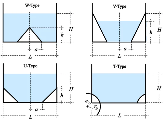
(43) Figure 2.3 Scheme of a rectangular tank The more complicated geometries are illustrated then in Figure 2.4. The first one is a W-Type Tank corresponding to a rectangular tank with a triangular obstacle located at the bottom, with its location and size defined by a and h as shown in the figure. The next two are the U-Type and V-Type Tanks, respectively, both corresponding to a tank with sloped walls, defined similarly through parameters a and h. The only difference is that the U-Type Tank satisfies the condition of h<H while the V-Type Tank satisfies the condition of h>H. The final one is the T-Type that corresponds to a tank where the inferior corners are rounded by semicircles defined by an eccentricity eo and a radius ro. Note that for all cases, H is the non-perturbed water depth and L is the length of the tank. Therefore the aspect ratio R= H/L can still be used to parameterize the tanks, establishing a uniformity with respect to the rectangular tank discussed earlier. Additionally, two new ratios are introduced for each type of tank to facilitate this parameterization corresponding to a normalization with respect to the external. 26.

(44) dimensions L and H: h = h / H and a = a / L / 2 for V-Tank, U-Tank and W-Tank, while r = ro / H and e = eo / ro for T-Tank.. Figure 2.4 Description of four different non-rectangular tank geometries, termed as Wtype, V-type, U-type and T-type tanks In general, the cross-section shape is defined by the following dimensionless ratios: (R) for rectangular tanks, ( h , a , R) for V-W-U-Tanks and ( r , e , R) for T-Tanks. Then, the incorporation of the length L allows scaling the shape to a particular size such that it is feasible to have tanks with the same shape but different sizes. The width of the tank (dimension out of plane) then sizes the overall liquid mass. 27.