AGNs and their host galaxies in the local universe : two mass independent Eddington ratio distribution functions characterize black hole growth

Texto completo

(1)The Astrophysical Journal, 845:134 (33pp), 2017 August 20. https://doi.org/10.3847/1538-4357/aa803b. © 2017. The American Astronomical Society. All rights reserved.. AGNs and Their Host Galaxies in the Local Universe: Two Mass-independent Eddington Ratio Distribution Functions Characterize Black Hole Growth Anna K. Weigel11 , Kevin Schawinski1. , Neven Caplar1. , O. Ivy Wong2,3. , Ezequiel Treister4,5,6, and Benny Trakhtenbrot1. Institute for Astronomy, Department of Physics, ETH Zurich, Wolfgang-Pauli-Strasse 27, CH-8093 Zurich, Switzerland 2 International Centre for Radio Astronomy Research, The University of Western Australia M468, 35 Stirling Highway, Crawley, WA 6009, Australia 3 ARC Centre for Excellence for All-Sky Astrophysics (CAASTRO), Australia 4 Instituto de Astrofísica, Facultad de Física, Pontificia Universidad Católica de Chile, 306, Santiago 22, Chile 5 EMBIGGEN Anillo, Concepcioń, Chile 6 Departamento de Astronomía Universidad de Concepcioń, Casilla 160-C, Concepcíon, Chile Received 2017 February 28; revised 2017 July 10; accepted 2017 July 15; published 2017 August 18. Abstract We use a phenomenological model to show that black hole growth in the local universe (z  0.1) can be described by two separate, mass-independent Eddington ratio distribution functions (ERDFs). We assume that black holes can be divided into two independent groups: those with radiatively efficient accretion, primarily hosted by optically blue and green galaxies, and those with radiatively inefficient accretion, which are mainly found in red galaxies. With observed galaxy stellar mass functions as input, we show that the observed active galactic nucleus (AGN) luminosity functions can be reproduced by using mass-independent, broken power-law-shaped ERDFs. We use the observed hard X-ray and 1.4 GHz radio luminosity functions to constrain the ERDF for radiatively efficient and inefficient AGNs, respectively. We also test alternative ERDF shapes and mass-dependent models. Our results are consistent with a mass-independent AGN fraction and AGN hosts being randomly drawn from the galaxy population. We argue that the ERDF is not shaped by galaxy-scale effects, but by how efficiently material can be transported from the inner few parsecs to the accretion disc. Our results are incompatible with the simplest form of mass quenching where massive galaxies host higher accretion rate AGNs. Furthermore, if reaching a certain Eddington ratio is a sufficient condition for maintenance mode, it can occur in all red galaxies, not just the most massive ones. Key words: galaxies: evolution – galaxies: luminosity function, mass function – quasars: supermassive black holes Our aim is to understand the effect of black holes on their host galaxies and vice versa on a global scale. To do so we introduce a model that allows us to put observations into context and to estimate and interpret their impact. Large galaxy surveys, such as the SDSS (York et al. 2000; Abazajian et al. 2009) or zCOSMOS (Lilly et al. 2007), allow us to examine the population in great detail. We are able to constrain the luminosity and stellar mass functions (at z ~ 0 e.g., Blanton et al. 2003; Pérez-González et al. 2008; Baldry et al. 2012; Moustakas et al. 2013; Moffett et al. 2016; Weigel et al. 2016 hereafter W16) and to study the evolution of the specific star formation rate (sSFR) distribution, which links the two (Sargent et al. 2012; Bernhard et al. 2014; Ilbert et al. 2014). For black holes, the equivalent to the sSFR distribution is the Eddington ratio distribution function (ERDF)7 The ERDF is the distribution of normalized black hole accretion rates (l = L bol LEdd ).8 While λ is an indicator of the small-scale accretion process, the ERDF describes the distribution of one of the fundamental black hole properties and represents a powerful population probe. In analogy to galaxies, the ERDF links the black hole mass function to the AGN luminosity function. While observationally constraining the AGN luminosity function is possible for a range of wavelengths, redshifts and luminosities (e.g., Ueda et al. 2003; Hasinger et al. 2005; Richards et al. 2006b;. 1. Introduction An active area of research in astrophysics today is the existence and extent of the galaxy–black hole connection. Assuming there is a causal link, are galaxies dictating the growth of black holes? Or is the energy of active galactic nuclei (AGNs) effective enough to impact galaxy evolution? Local scaling relations between black holes and their host galaxies (e.g., Kormendy & Richstone 1995; Magorrian et al. 1998; Ferrarese & Merritt 2000; Gebhardt et al. 2000; Tremaine et al. 2002; Marconi & Hunt 2003; Gültekin et al. 2009; Kormendy & Ho 2013a; Graham 2016; Savorgnan & Graham 2016) are often attributed to galaxy–black hole co-evolution (see e.g., Silk & Rees 1998; Fabian 1999; King 2003; Di Matteo et al. 2005), but they could also have a non-causal origin, for instance galaxy–galaxy mergers (Peng 2007; Jahnke & Macciò 2011). Besides the local scaling relations, the similar redshift evolution of the star formation rate density and the black hole accretion rate density points toward a possible galaxy–black hole connection (e.g., Boyle & Terlevich 1998; Heckman et al. 2004; Hasinger et al. 2005; Silverman et al. 2009; Mullaney et al. 2012). Furthermore, the effect of AGNs on their host galaxies in the form of feedback is associated with the quenching of star formation (Sanders et al. 1988; Di Matteo et al. 2005; Cattaneo et al. 2009; Fabian 2012) and could explain the observed bi-modality in color–magnitude and color–mass space (Bell et al. 2003; Baldry et al. 2004; Faber et al. 2007; Martin et al. 2007; Schawinski et al. 2014). The galaxy–black hole connection thus seems complex and multifaceted, especially if we consider additional aspects such as galaxy morphology and redshift evolution.. 7. Note that this is only approximately true. The sSFR direcly corresponds to the stellar mass e-folding time. However, deriving the black hole mass efolding time from the Eddington ratio requires the assumption of the radiative efficiency. 8 Throughout the paper we will be referring to λ as the Eddington ratio.. 1.

(2) The Astrophysical Journal, 845:134 (33pp), 2017 August 20. Weigel et al.. Bongiorno et al. 2007; Hopkins et al. 2007; Aird et al. 2015; Miyaji et al. 2015), measuring reliable black hole masses and their distribution for a large sample is more complex (Trakhtenbrot & Netzer 2012; Shen 2013; Peterson 2014; Mejía-Restrepo et al. 2016). In previous work, the black hole mass function and the corresponding Eddington ratio values have been measured observationally (Heckman et al. 2004; McLure & Dunlop 2004; Kollmeier et al. 2006; Kauffmann & Heckman 2009; Schulze & Wisotzki 2010; Trump et al. 2011; Aird et al. 2012, 2017; Bongiorno et al. 2012; Kelly & Merloni 2012; Lusso et al. 2012; Nobuta et al. 2012; Shen & Kelly 2012; Schulze et al. 2015; Bongiorno et al. 2016; Jones et al. 2016) and have been studied using a phenomenological approach (Merloni et al. 2004; Shankar et al. 2004, 2009, 2013; Yu & Lu 2004; Merloni & Heinz 2008; Hopkins & Hernquist 2009; Shen 2009; Cao 2010; Li et al. 2011; Conroy & White 2013; Novak 2013; Veale et al. 2014; Aversa et al. 2015; Caplar et al. 2015; Tucci & Volonteri 2017). We present the results of a phenomenological model that links the galaxy and black hole populations in the local universe (z  0.1). The purpose of this analysis is not to infer from the data what the ERDF’s properties are, as some studies have done (e.g., Kollmeier et al. 2006; Shen et al. 2008; Kauffmann & Heckman 2009; Schulze & Wisotzki 2010; Aird et al. 2012; Jones et al. 2016), but rather to forward model the process: if we assume a certain, simple ERDF shape, how far can we go in characterizing the AGN population? Our aim is to make the simplest and most straightforward assumptions possible. These assumptions might not be exactly true, but they do allow us to make inferences about black hole growth on a global scale. For example, we assume that AGNs can be separated into two independent populations: those that accrete radiatively efficiently and are primarily found in optically blue and green galaxies, and those with radiatively inefficient accretion that are mostly found in optically red, quiescent galaxies (Fabian 2012; Kormendy & Ho 2013b; Heckman & Best 2014). Starting from the galaxy stellar mass function, we predict the black hole mass function and AGN luminosity function by assuming an ERDF. This ERDF is assumed to have a broken power-law shape and to be mass independent. We test whether the observed AGN luminosity functions, in the X-rays for radiatively efficient AGNs and in the radio for radiatively inefficient AGNs, can be reproduced with this simple model, and constrain the corresponding ERDFs. We discuss the physical implications of our results in the context of mass quenching (Sanders et al. 1988; Di Matteo et al. 2005; Cattaneo et al. 2009; Peng et al. 2010, 2012; Fabian 2012), maintenance mode (Croton et al. 2006; Bower et al. 2006; Springel et al. 2006; Somerville et al. 2008; Fabian 2012) and black hole growth in general. The paper is structured as follows. In Section 2 we introduce our model. After having discussed our assumptions, we establish our method in Section 3. Section 4 summarizes the application of the method to the observations and our results. We examine the implications of these results in Section 5. In Section 6 we discuss variations and caveats of our model and compare our results to previous work. We conclude this paper with a summary in Section 7. Throughout this paper, we denote the logarithm to base 10 as log and assume a ΛCDM cosmology with h 0 = 0.7, Wm = 0.3 and WL = 0.7 (Komatsu et al. 2011).. Figure 1. AGN radio and X-ray luminosity functions. Shown on the right-hand side of this figure are the hard X-ray luminosity functions (XLFs) from A12 (15–55 keV), Tueller et al. (2008) (14–195 keV), and Sazonov et al. (2007) (17–60 keV). The 1.4 GHz radio luminosity functions (RLF) from MS07 and Pracy et al. (2016) are illustrated on the left-hand side. To allow for an easier comparison between the RLF and the XLF we converted the radio luminosities from W Hz-1 to erg s-1. Compared to the RLF, the XLF is significantly steeper and has a pronounced break.. 2. Model and Assumptions The ERDF, x (l ), describes the distribution of Eddington ratios of a black hole population. It shows what fraction of black holes have Eddington ratios within a certain range and thus links the black hole mass function to the AGN luminosity function. As we have discussed above, the black hole population is linked to the galaxy population through local scaling relations. By correlating the stellar mass and black hole mass functions, the shape of the AGN luminosity function can hence be traced back to the ERDF and the stellar mass function (Caplar et al. 2015, hereafter C15). Our aim is to test if the observed AGN luminosity function can be reproduced by a simple model. Instead of starting with the AGN luminosity function and inferring the ERDF, we use a forward modeling approach and base our model on the underlying galaxy population and its stellar mass function. We assume that the ERDF is mass independent and broken power-law shaped, test if this ERDF allows us to reproduced the observed AGN luminosity function, and constrain the ERDF’s parameters. In Figure 1 we show the hard X-ray luminosity function (XLF) from Ajello et al. (2012) (hereafter A12) and the 1.4 GHz radio luminosity function (RLF) from Mauch & Sadler (2007) (hereafter MS07) which we use to compare our predictions with the observations. For the RLF we converted the 1.4 GHz radio luminosity from W Hz-1 to erg s-1 to allow for an easier comparison with the XLF. The figure shows that, compared to the XLF, the RLF is significantly shallower. The shape of the AGN luminosity function depends on the shape of the stellar mass function and the ERDF. Yet even if we use different stellar mass functions as input, due to their significantly different shapes we are unable to reproduce both the XLF and the RLF with a single ERDF. Different ERDF shapes indicate that, in our model, radio 2.

(3) The Astrophysical Journal, 845:134 (33pp), 2017 August 20. Weigel et al.. and X-ray AGNs cannot be considered as being part of the same black hole growth mode. Therefore our first assumption is the following.. low levels of radio emission, can thus also be detected using selection methods based on, for example, X-ray (Wong et al. 2016) or infrared (Hardcastle et al. 2013) emission. Bright HERGs are often referred to as radio-loud quasars. Heckman & Best (2014) show that below log (P1.4 GHz W Hz-1) = 26 the space density of LERGs is significantly higher than that of HERGs (also see Best & Heckman 2012; Gendre et al. 2013; Heckman & Best 2014; Pracy et al. 2016). While HERGs become dominant at high radio luminosities, their space density is several orders of magnitude lower than that of LERGs at, for example, log (P1.4 GHz W Hz-1) = 22. The number of radio AGNs that accrete via radiatively efficient accretion is thus negligible. For our model we neglect this overlap between the radiatively efficient and inefficient AGN populations and consider X-ray and radio AGNs separately. We furthermore assume that they are detected in the hard X-rays and at 1.4 GHz, respectively.. 1. In the local universe AGNs can be separated into radiatively efficient and inefficient AGNs, detected in the hard X-rays and at 1.4 GHz, respectively. The two groups show little overlap, can be treated separately, and each has a characteristic ERDF. We discuss the need for two separate ERDFs in more detail in Section 5.1. We make additional assumptions to link the black hole and galaxy populations and to be able to compare our predicted AGN luminosity functions with the observations. We stress that these assumptions are intended to describe the galaxy and black hole populations on a global scale. They might not be able to capture all underlying complexities, but are meant to be as simple as possible, broadly true, and sufficient to infer general relations. We assume. 2.2. The Host Galaxies of Radiatively Efficient AGNs. 2. that radiatively efficient AGNs are primarily found in optically blue and green galaxies, 3. a constant bolometric correction for the hard X-rays of kbol,X = log (LX L bol ) = -1, 4. that radiatively inefficient AGNs are mostly hosted by optically red, quiescent galaxies, 5. a constant bolometric correction for 1.4 GHz of kbol,R = log (LR L bol ) = -3, 6. a constant MBH - Mhost scaling relation to convert stellar into black hole masses (log (MBH M ) = -2.75, scatter 0.3 dex), 7. that both the ERDFs for radio AGNs and X-ray AGNs are mass independent and broken power-law shaped.. In the local universe, the bimodality that we observe in color–mass and color–magnitude space is well established (Bell et al. 2003; Baldry et al. 2004; Faber et al. 2007; Martin et al. 2007; Schawinski et al. 2014). On one hand, star-forming galaxies, which are predominantly late-type/disc dominated, inhabit the “blue cloud.” On the other hand, quiescent galaxies, mostly early type and/or bulge dominated, are found on the “red sequence.” Between these two populations lies the transition zone, the “green valley” (Bell et al. 2004; Martin et al. 2007; Fang et al. 2012; Schawinski et al. 2014). Previous work has shown that X-rayselected AGNs are found in galaxies that show signs of star formation, so either in the blue cloud or the green valley (Hickox et al. 2009; Schawinski et al. 2009; Silverman et al. 2009; Treister et al. 2009; Koss et al. 2011; Rosario et al. 2013; Goulding et al. 2014). For our simple model we assume that most of the X-rayselected AGNs are hosted by blue and green galaxies and use the stellar mass function of these galaxies as input when constraining the ERDF relative to the XLF.. We will now discuss each of these assumptions in more detail. 2.1. Two Accretion Modes We assume that active black holes can be observed in two distinct accretion modes: radiative and radio mode. In the radiative mode, AGNs accrete via a geometrically thin, optically thick accretion disc (e.g., Shakura & Sunyaev 1973). The Eddington ratio and the radiative efficiency of these AGNs are of the order of 10%, i.e., the potential energy of the infalling matter is efficiently converted to radiation. In contrast, AGNs that are in the radio mode have a low radiative efficiency and low Eddington ratios. Their accretion flows are geometrically thick and optically thin, which results in a radiative cooling time that is longer than the infall time (Narayan & Yi 1994; Narayan & McClintock 2008). Radio or jet mode AGNs are often found in massive, red elliptical galaxies (e.g., Best et al. 2005), whereas radiative or quasar mode AGNs tend to be hosted by galaxies with bluer colors and higher SFRs (see discussion below and e.g., Nandra et al. 2007; Hickox et al. 2009; Netzer 2009; Schawinski et al. 2009; Treister et al. 2009; Griffith & Stern 2010; Goulding et al. 2014). The two AGN populations show an overlap in the form of highexcitation radio galaxies. Based on optical emission lines, radio galaxies can be split into high- and low-excitation radio galaxies (HERGs and LERGs, Hardcastle et al. 2006, 2007; Smolčić 2009; Heckman & Best 2014; Ching et al. 2017). The distinction is linked to different AGN accretion modes (Hardcastle et al. 2006; Smolčić 2009): HERGs accrete via radiatively efficient accretion, whereas LERGs accrete via radiatively inefficient, advectiondominated accretion. HERGs, which are similar to Seyferts with. 2.3. Bolometric Correction for Hard X-Ray-selected AGNs To be able to compare our predicted to the observed XLF, we need to convert from bolometric to hard X-ray luminosities. Although the spectral energy distributions of AGNs show a high degree of uniformity from the X-rays to the infrared (Elvis et al. 1994; Richards et al. 2006a), previous studies have suggested that the X-ray bolometric correction might be luminosity or Eddington ratio dependent (Marconi et al. 2004; Hopkins et al. 2007; Vasudevan & Fabian 2009; Lusso et al. 2010, 2012). We consider the simplest model and assume a constant bolometric correction. We discuss the effect that a luminosity-dependent bolometric correction would have on our results in Appendix B.2. Rigby et al. (2009) determine L17 – 60 keV L 2 – 10 keV to be 1.34. We use the same value to convert from 15–55 keV to 2–10 keV. Averaging over a wide range of Eddington ratios, we assume L bol L 2 – 10 keV = 20 based on the results by Vasudevan & Fabian (2009). We conclude: log L15 - 55 keV = log L bol - log k soft - bol - log k hard - soft  log L bol - log 20 + log 1.34 ⎛L erg s-1 ⎞ k bol,X = log ⎜ 15 - 55 keV -1 ⎟ = - 1. ⎠ ⎝ L bol erg s. 3. (1 ).

(4) The Astrophysical Journal, 845:134 (33pp), 2017 August 20. Weigel et al.. Jahnke et al. (2009, μ = −2.75), Kormendy & Ho (2013b, μ = −2.31), McConnell & Ma (2013, μ = −2.54), Marleau et al. (2013, μ = −3.02) and Reines & Volonteri (2015, μ = −3.55). We do not take into account variations in the relation that might arise due to different levels of star formation, different morphological classifications, or using bulge instead of total stellar mass (Sani et al. 2011; Reines & Volonteri 2015; Savorgnan et al. 2016; Terrazas et al. 2016), and we use stellar mass M for the host mass Mhost.. 2.4. The Host Galaxies of Radiatively Inefficient AGNs In our model we assume that the 1.4 GHz RLF is produced by radiatively inefficient AGNs which are hosted by red, quiescent galaxies. The fact that low Eddington ratio radio AGNs are primarily found in massive ellipticals is well established (Matthews et al. 1964; Yee & Green 1987; Best et al. 2005; Hickox et al. 2009). The HERG and LERG distinction has been introduced more recently (Hardcastle et al. 2006, 2007; Smolčić 2009; Heckman & Best 2014). As we discussed above, the RLF is dominated by LERGs which accrete via radiatively inefficient accretion. These LERGs are predominantly hosted by optically quiescent, red galaxies (Smolčić 2009; Smolčić et al. 2009; Janssen et al. 2012; Ching et al. 2017).. 2.7. A Broken Power-law-shaped ERDF While alternative ERDF shapes have been discussed previously (Kollmeier et al. 2006; Kauffmann & Heckman 2009; Hopkins & Hernquist 2009; Cao 2010; Aird et al. 2012, 2013a; Bongiorno et al. 2012, 2016; Nobuta et al. 2012; Conroy & White 2013; Hickox et al. 2014; Veale et al. 2014; Schulze et al. 2015; Trump et al. 2015; Jones et al. 2016), we assume a broken power-lawshaped ERDF for both radiatively efficient and inefficient AGNs. A broken power-law-shaped ERDF solves the apparent discrepancy between a Schechter function-shaped stellar mass function and an observed broken power-law-shaped luminosity function. Furthermore, a broken power-law-shaped ERDF allows us to change both the high and the low Eddington ratio end slopes. Besides a functional form for the ERDF, we assume that the ERDF is mass independent. Mass-dependent ERDFs have been proposed (Schulze et al. 2015; Bongiorno et al. 2016), yet not introducing a mass dependence constitutes a straightforward first assumption. In Sections 4.3 and 6.1 we discuss a possible mass dependence and alternative ERDF shapes, respectively.. 2.5. Bolometric Correction for Radio AGNs To convert our predicted bolometric luminosity functions to 1.4 GHz, we use a constant bolometric correction of ⎛L erg s-1 ⎞ k bol,R = log ⎜ 1.4 GHz ⎟ = - 3. ⎝ L bol erg s-1 ⎠. (2 ). This is a simplified assumption since the connection between the AGN bolometric luminosity and the 1.4 GHz core emission is complex. First of all, radio loudness  , i.e., the ratio of radio to optical emission, is a function of the Eddington ratio (Woo & Urry 2002; Ho 2002); the higher λ, the lower the radio loudness. Depending on whether the total or only the core radio luminosity is taken into account, there is furthermore evidence for (Sikora et al. 2007) and against (Broderick & Fender 2011) a radio-loud/ radio-quiet dichotomy in  - l space. In addition, radio AGNs release energy in the form of mechanical jet power and so only a fraction of their total energy is emitted in the form of radiation (Falcke & Biermann 1995; Bîrzan et al. 2004, 2008; Körding et al. 2008; Cattaneo & Best 2009; Cavagnolo et al. 2010; Plotkin et al. 2012; Turner & Shabala 2015; Godfrey & Shabala 2016; Mingo et al. 2016). To constrain the shape of x (l ), we need to propose a kbol,R value. Motivated by the fact that radio AGNs, specifically LERGs, tend to have low Eddington ratios compared to radiatively efficient AGNs or HERGs (Ho 2002; Evans et al. 2006; Hardcastle et al. 2007; Merloni & Heinz 2008; Hickox et al. 2009; Smolčić 2009; Alexander & Hickox 2012; Best & Heckman 2012; Fabian 2012), we choose kbol,R = -3. We stress that we do not claim kbol,R to be precisely −3. This value represents an assumption which allows us to test whether the observed RLF is consistent with a mass-independent ERDF and a constant bolometric correction. While summarizing all complexities that affect kbol,R into a single constant allows us to constrain the shape of the radio ERDF, we do not claim to be able to determine the absolute value of the ERDF break, as we will discuss in more detail below.. 3. Method After introducing our assumptions in the previous section, we now discuss our method. This relies on an input stellar mass function and an assumed ERDF. We parameterize the single Schechter (Schechter 1976) stellar mass function in the following functional way: (4 ). Here, the factor of ln (10) and the +1 in the power-law exponent are due to the conversion from dM to d log M . Similarly the double Schechter function is given by: F (M ) =. dN d log M. ⎛ M ⎞ ⎡ ⎛ M ⎞a1+ 1 ⎛ M ⎞a2 + 1⎤ ⎟ ⎢F* ⎜ ⎟ ⎜ ⎟ * = ln (10) exp ⎜ + F ⎥. 2 ⎝ M* ⎠ ⎣ 1 ⎝ M* ⎠ ⎝ M* ⎠ ⎦ (5 ). As we assume that the ERDF is broken power-law shaped and mass independent, we parameterize the broken power-law ERDF in the following way:. 2.6. The Local MBH –Mhost Relation To convert stellar to black hole masses, we use the local MBH –Mhost scaling relation. We parameterize the relation as ⎛M ⎞ ⎛M ⎞ log ⎜ BH ⎟ = m + b ´ log ⎜ host ⎟ ⎝ M ⎠ ⎝ M ⎠. ⎛ M ⎞a+ 1 ⎛ M ⎞ dN ⎟ ⎟. exp ⎜ = ln (10) F*⎜ ⎝ ⎠ ⎝ M* ⎠ * d log M M. F (M ) =. x (l ) =. (3). dN = x* ´ (N dlogl). ⎡⎛ l ⎞d1 ⎛ l ⎞d2 ⎤-1 ⎢⎜ ⎟ + ⎜ ⎟ ⎥ ⎝ l* ⎠ ⎦ ⎣⎝ l* ⎠. (6 ). and define d1 and d2 as the low and high Eddington ratio slopes, respectively. With F(M ) and x (l ) as input, we can predict the AGN bolometric luminosity function, FL (L ), which is. and choose μ = −2.75, β = 1 and σ = 0.3 dex. This μ value lies between the results of Häring & Rix (2004, μ = −2.8), 4.

(5) The Astrophysical Journal, 845:134 (33pp), 2017 August 20. Weigel et al.. commonly parameterized as a broken power law of the form: FL (L ) =. ⎞g2 ⎤-1. ⎡⎛ L ⎛L dN = A ´ ⎢⎜ ⎟ + ⎜ ⎟ ⎥ . ⎝ ⎠ ⎝ L* ⎠ ⎦ ⎣ d log L L* ⎞g1. 3. Convert all stellar masses to black hole masses by assuming a conversion factor μ with scatter σ: We assume the local MBH –Mhost relation (see Section 2.6) and draw Ndraw conversion factors from a normal distribution with mean m = log MBH M = -2.75 and scatter s = 0.3. log MBH is then given by the sum of these conversion factors and the previously drawn stellar mass values. Having determined log MBH allows us to construct the black hole mass function. We bin in log MBH and adjust the normalization so that log FBH in bin i is given by. (7 ). g1 represents the faint and g2 the bright end of the luminosity function. With the appropriate bolometric corrections, we can then compare our prediction with the observed XLF or RLF. We introduce two manifestations of our method: the first is based on random draws (see Section 3.1), whereas for the second we employ multiple convolutions (see Section 3.2). In Section 3.3 we discuss the properties of the predicted luminosity function. To constrain the ERDFs of radiatively efficient and inefficient AGNs we use a Markov chain Monte Carlo (MCMC) sampler which we introduce in Section 3.4. We also discuss our model in the context of key terms such as “variability,” “occupation fraction,” “duty cycle,” and “active black hole fraction” (Section 3.5). Figures 2 and 3 summarize the random draw and the convolution method and all relevant parameters. The results of the two methods, which we introduce below, are equivalent, but differ in their computational expense. The random draw approach is computationally more expensive, but more easily adjusted. For instance, we use the random draw method to demonstrate the effects of a mass-dependent ERDF (see Section 4.3). The convolution approach is computationally less expensive and thus used to constrain the ERDF shape with an MCMC.. ⎞ ⎛ ni log FBH, i = log ⎜ ⎟. ⎝ V (zmin , zmax , W) ´ D log MBH ⎠. Here, ni corresponds to the number of simulated systems in bin i, V (zmin, zmax, W) is the volume that we have already used in Equation (8) and D log MBH represents the bin size. 4. Construct the CDF of the ERDF and draw Eddington ratio values log l : We also assign randomly drawn Eddington ratio values to black hole mass value. In analogy to Equation (9) we construct the CDF for the given ERDF in the range log lmin to log lmax . The shape of the CDF is not affected by the normalization of the ERDF. However x * determines how many of the Ndraw black hole mass values are assigned an Eddington ratio value. If the integral over x (l ) from log lmin to log lmax is 1 we draw Ndraw log l values from the CDF. However, if the integral over the ERDF is a with a < 1, then only Ndraw,AGN = a ´ Ndraw black holes are assigned a log l value. 5. Calculate bolometric luminosities to determine FL (L bol ): We compute the bolometric luminosities corresponding to the Ndraw,AGN black holes and their corresponding log l values:. 3.1. The Random Draw Method Our first method to predict the bolometric luminosity function is based on random draws and is illustrated in the top panels of Figure 3. We use a stellar mass function and an ERDF as input and perform the following steps. 1. Determine Ndraw: Before drawing from the stellar mass function, we need to determine the number of values to be drawn, Ndraw. This is a simple scaling factor which determines the lowest number densities that we can probe with the random draw method. Ndraw can be given a physical meaning by linking it to the stellar mass function. For example Ndraw can be defined as: Ndraw = V (zmin , zmax , W) ´. log Mmax. òlog M. F (M ) d log M .. (10). log (L bol erg s-1) = log l + log (MBH M) + r.. Here, r = log. (. LEdd erg s-1 MBH M. (11). ) = 38.2. In analogy to the. black hole mass function, we bin in log L bol . log FL in bin i is then given by:. (8 ). min. Here, log Mmin and log Mmax denote the minimum and maximum stellar mass values that we consider in the draw, respectively. V (zmin, zmax, W) can be chosen to represent the comoving volume (e.g., Hogg 1999) of a specific survey with solid angle Ω. 2. Construct the cumulative distribution function (CDF) of the stellar mass function and draw stellar mass values: After having determined Ndraw, we construct the CDF of the stellar mass function by computing:. ⎞ ⎛ ni log FL, i = log ⎜ ⎟. ⎝ V (zmin , zmax , W) ´ D log L bol ⎠. (12). 3.2. The Convolution Method. (9 ). Our second method to predict the shape of the luminosity function is based on convolutions and follows the work of C15. We again use a stellar mass function and an ERDF as input and go through the following steps (see the bottom row of Figure 3):. We randomly draw Ndraw numbers between 0 and 1 from a uniform distribution and, by inverting CDF (log M ), assign the corresponding stellar mass values.. 1. Convolve the stellar mass function with a normal distribution to predict the black hole mass function: We convolve the observed stellar mass function with a normal distribution with mean μ and standard deviation. log M. CDF(log M ) =. òlog Mmin F (M ) d log M log M. max òlog Mmin F (M ) d log M. .. 5.

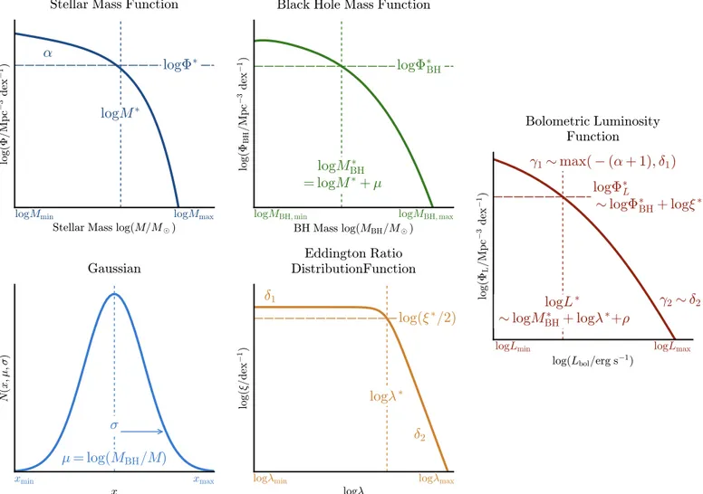
(6) The Astrophysical Journal, 845:134 (33pp), 2017 August 20. Weigel et al.. Figure 2. Overview of the most important parameters and variables used in our model. The stellar mass function is described as a standard single or double Schechter function with break log M *, slope α and normalization Φ (see Equations (4) and (5)). We construct the black hole mass function FBH from the stellar mass function by assuming a constant log MBH to log M ratio μ with log-normal scatter σ (see Sections 3.1 and 3.2). We assume a broken power-law Eddington ratio distribution function x (l ) with break log l* and slopes d1 and d 2 . We describe the luminosity function as a broken power law with break log L*, normalization F*L , faint end slope g1, and bright end slope g2 (see Equation (7)). In Section 3.3 we discuss how log L*, g1, and g2 are related to the stellar mass function and Eddington ratio distribution function parameters.. σ:. x (l ): FL (log L ) = (FL,log l = 0 * x )(log L ). FBH (log MBH) = (F * N )(log MBH) =. log Mmax. òlog M. =. [F (log M ). min. [FL,log l = 0 (log L - log l). min. ´ x (log l)] d log l.. ´ N (log MBH - log M , m , s )] d log M . (13). Here, N (x, m, s ) is the normal distribution and F(M ) is the stellar mass function which is described by either a single or a double Schechter function (see Equations (4) and (5)). 2. Convolve the predicted black hole mass function with the given ERDF to determine the shape of the bolometric luminosity function: First, we assume a constant Eddington ratio of log l = 0 and shift FBH (log MBH ) from black hole mass to bolometric luminosity space FL,log l= 0 (log L ) = FBH (log MBH + r ).. log l max. òlog l. (15). Besides the ERDF parameters, both the random draw and the convolution method require choices for log Mmin , log Mmax , log lmin and log lmax . We use log (Mmin M) = 9 and log (Mmax M) = 12 since this is the mass range over which the W16 stellar mass functions are constrained. We discuss the effect of this choice on our results in Appendix B.1. We set log lmin and log lmax to −8 and 1, respectively (also see Table 2). The values of log lmin and log lmax are degenerate with the normalization of the ERDF. x * determines what fraction of black holes are assigned an Eddington ratio between log lmin and log lmax and can therefore be considered as being “on” (see Section 3.5). In the framework of the random draw technique, assigning log l values to all Ndraw black hole mass values implies that all black holes in the sample can be considered AGNs. The. (14). To take into account the fact that the Eddington ratio is not constant, we convolve FL,log l= 0 with the ERDF, 6.

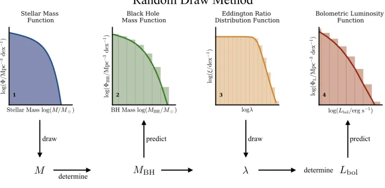
(7) The Astrophysical Journal, 845:134 (33pp), 2017 August 20. Weigel et al.. Figure 3. Schematic illustrating the two equivalent methods to predict the bolometric luminosity function shape. For both techniques we use an observed stellar mass function as input and assume an Eddington ratio distribution function. By applying constant bolometric corrections our predicted luminosity functions can then be compared to observed X-ray and radio luminosity functions. Our first method, which is based on a random draw (see Section 3.1), is illustrated in the upper panels. We randomly draw stellar mass values from the input stellar mass function (panel 1) and convert these to black hole masses, assuming a constant log MBH to log M ratio μ with log-normal scatter σ. Furthermore, we randomly draw Eddington ratio values from the input Eddington ratio distribution function x (l ) (panel 3). This allows us to not only predict the the black hole mass function (panel 2), but also the shape of the bolometric luminosity function (panel 4). The second technique is summarized in the lower panels. It is computationally less expensive since it is based on convolutions (see Section 3.2). We convolve the input stellar mass function (panel (a)) with a normal distribution with mean μ and standard deviation σ (panel (b)) to predict the black hole mass function (panel (c)). To determine the shape of the bolometric luminosity function (panel (e)), we convolve FBH with the Eddington ratio distribution function (panel (d)).. 7.

(8) The Astrophysical Journal, 845:134 (33pp), 2017 August 20. Weigel et al.. g1 = -(a + 1) we will not be able to constrain d1 well, since it can take any value d1 < -(a + 1). 3. The break L*: Under the assumption of d1 < a + 1, the position of the break of the luminosity function is given by:. convolution method produces the same result if the integral over x (l ) from log lmin to log lmax is 1. Without a priori knowledge of x * for the chosen log lmin and log lmax boundaries only the shape of the bolometric luminosity function, but not its normalization F*L , can be predicted. As we will discuss in more detail below, we determine x * by rescaling the predicted luminosity function so that the space density over the considered luminosity range matches the observed space density. Once we have determined the bolometric luminosity function through either the random draw or the convolution method, we use the bolometric corrections kbol,X and kbol,R to predict the XLF and the RLF. In both cases, this results in a constant shift toward lower luminosities since our assumed bolometric corrections are constant with luminosity and Eddington ratio. We discuss the effect of a luminosity-dependent bolometric correction in Appendix B.2.. * + log l* + r + log DL (d1, g2) log L* = MBH = M * + m + log l* + r + log DL (d1, g2).. Here, DL (d1, g2 ) is a small correction factor which is weakly dependent on the choice of d1 and g2 and varies by less than 0.15 dex. 4. The normalization F*L : At L* the normalization of the luminosity function can be predicted using log F*L = log F*BH + log x * + log DF (d1, g2) = log F* + log x * + log DF (d1, g2).. 3.3. The Predicted Luminosity Function. 3.4. MCMC The discussion in the previous section shows that we are likely to find ERDF parameters that allow us to reproduce the observed XLF and RLF. To constrain the best-fitting parameters for xX (l ) and xR (l ) and to quantify the corresponding uncertainties, we introduce an MCMC sampler. We use the broken power-law ERDF defined in Equation (6) and postulate d2 > d1. This ensures a predicted luminosity function shape similar to the observations and prevents the MCMC sampler from jumping between equivalent solutions during the sampling process. To incorporate this prior, we parameterize the broken power-law ERDF in the following way:. 1. The bright end slope g2 : C15 use a simplified ERDF with x () = 0 for log l < log l* to show how the x (l ) shape affects the predicted luminosity function. They show analytically that the bright end of the luminosity function has the same slope as the high λ end of the ERDF, that is: (16). As the stellar mass function falls off exponentially at high stellar masses, the shallower d2 slope is necessary to reproduce the observed bright end of the luminosity function. To construct the black hole mass function, we convolve the stellar mass function with a normal distribution. In contrast to the stellar mass function, the black hole mass function therefore no longer falls off exponentially at the high-mass end. In the extreme case, in which d2 is steeper than the exponential cut off of FBH , it is thus the high-mass end of the black hole mass function and not d2 that dominates g2 . 2. The faint end slope g1: The faint end of the luminosity function is determined by either the stellar mass function low-mass end slope α or the ERDF low Eddington ratio end slope, d1. Using their simplified model C15 conclude that g1 = -(aBH + 1). Here, aBH is the black hole mass function slope. If d1 is steeper than aBH + 1, the ERDF slope determines g1. The linear relation which we assume between M and MBH ensures that the stellar and black hole mass functions have the same low-mass end slopes. With aBH = a we hence conclude9 g1 = max [ - (a + 1) , d1].. (19). x * is the normalization of the ERDF and we have used the fact that in our model F = FBH . To derive this relation, C15 have again assumed d1 < a + 1 and introduced DF (d1, g2 ), a small correction factor which is dependent on d1 and g2 and varies by less than 0.15 dex.. Both methods allow us to predict the bolometric luminosity function once we have assumed the shape of x (l ). As we discussed above, a broken power-law shape is an appropriate first assumption for the ERDF since, in contrast to the stellar mass function, the observed AGN luminosity function is also power-law shaped. C15 derive and discuss the properties of the predicted luminosity function if a broken power-law-shaped ERDF is assumed. We summarize these characteristics of FL (L ) and its dependence on F(M ) and x (l ) below and in Figure 2.. d2 = g2.. (18). d2 = d1 +  ,  > 0 x (l ) =. dN = x* ´ (N d logl). ⎡⎛ l ⎞d1 ⎛ l ⎞d1+  ⎤-1 ⎢⎜ ⎟ + ⎜ ⎟ ⎥ . ⎝ l* ⎠ ⎣⎝ l* ⎠ ⎦. (20). We use the MCMC PYTHON package COSMOHAMMER10 (Akeret et al. 2013) to vary d1, ò, and log l*. In each step, the MCMC proposes a new set of ERDF parameters. We use this prediction for the ERDF and the input stellar mass function to estimate the corresponding bolometric luminosity function FL,pred with the convolution technique. To shift the luminosity function to the hard X-ray or the 1.4 GHz radio regime we apply a constant bolometric correction. We then determine the predicted space densities (FL,pred ) in the luminosity bins of the observed luminosity function (log L obs). The normalization of the ERDF, x * is degenerate with log l*, d1 and d2 . To minimize the number of free parameters and degeneracies, we do not include x * in the MCMC. Instead we rescale FL,pred so that the space densities of the predicted and the observed luminosity functions match: ˜ L,pred = n obs ´ FL,pred . F (21) n pred. (17). Equation (17) shows that for luminosity functions with 9 Our definition of α differs from that used by C15. In our case, a flat Schechter function has a slope of a = -1, whereas they use a = 0 . We are thus defining g1 in terms of a + 1.. 10. 8. http://cosmohammer.readthedocs.org/.

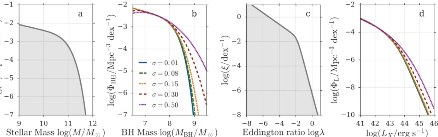
(9) The Astrophysical Journal, 845:134 (33pp), 2017 August 20. Weigel et al.. Figure 4. Effect of the log M - log MBH ratio scatter and the resulting black hole mass function shape on the predicted luminosity function. Panel (a) shows the blue+green stellar mass function which we use as input. We convert F(log M ) to the black hole mass function, which is shown in panel (b), by convolving it with a normal distribution. This has a mean μ and a standard deviation σ where we vary σ. We convolve all black hole mass functions with the same ERDF, shown in panel (c), to predict the corresponding X-ray luminosity functions, which are shown in panel (d). This figure illustrates that the bright end of the luminosity function, g2 , is determined by either the high-mass end of the black hole mass function or the high Eddington ratio end of the ERDF. For s  0.15, the high-mass end of the black hole mass function is steeper than d 2 . g2 of all black hole mass functions with s  0.15 is thus independent of σ and solely determined by d 2 . For s > 0.15, the black hole mass function is shallower than the ERDF. g2 is therefore given by the high-mass end of the black hole mass function, which depends on the assumed σ. The input stellar mass function and the assumed ERDF determine the σ value above which g2 is no longer affected by d 2 .. Here nobs and n pred represent the integrals over the predicted and the observed luminosity functions within the observed luminosity function’s binning range. To compute the log-likelihood for each set of new ERDF parameters, we use the observed log FL,obs values and their errors and the predicted log FL,pred values in the log L obs bins. We assume that the asymmetric observed errors on log FL,obs follow a log-normal distribution and describe the details of the ln  calculation in Appendix A.1. Once the MCMC has converged we use the MCMC chain to determine the median log l*, d1 and ò values and the corresponding 16 and 84 percentiles. Using the definition of ò in Equation (20), we determine the sum of the d1 and the ò chains to estimate the median d2 value and its credible intervals. It is important to acknowledge that the shape of the predicted luminosity function will not be affected by d1 values that lie significantly below -(a + 1). According to Equation (17), g1 will be given by α, the low-mass end of the stellar mass function, if d1  -(a + 1). So, if d1 ~ -(a + 1), we have to interpret d1 as an upper limit. We can only fully constrain d1, if g1 is significantly steeper than the stellar mass function (g1  -(a + 1)). As we have pointed out in Section 3.3, g2 does not solely rely on d2 , but is also affected by the steepness of the black hole mass function. We illustrate this effect in Figure 4. We vary the scatter in the stellar to black hole mass conversion by convolving the blue+green stellar mass function (panel (a)) with normal distributions with different widths σ. The corresponding black hole mass functions (panel (b)) are then all convolved with the same ERDF (panel (c)) to estimate the corresponding XLFs (panel (d)). Figure 4 illustrates that for low σ values the shape of the black hole mass function does not affect the shape of FL ; it is d2 that determines g2 . For high σ values, d2 is however irrelevant and g2 depends on the shallower high-mass end of the black hole mass function.. 3.5. Variability, Occupation Fraction, Duty Cycle, and Active Black Hole Fraction In this section, we discuss how in our model the normalizations of the stellar mass function, black hole mass function, and the ERDF are linked to the black hole occupation fraction, the fraction of active black holes, and the duty cycle. 1. Black hole occupation fraction: We define the black hole occupation fraction as the fraction of galaxies that are hosting a black hole. In the local universe most massive galaxies, including our own, host a black hole (Genzel et al. 1996; Ghez et al. 2000, 2008; Magorrian et al. 1998; Schödel et al. 2003). In our model, we thus assume an occupation fraction of 100%. At high redshift the occupation fraction might however be lower than 100% (Treister et al. 2013; Weigel et al. 2015; Trakhtenbrot et al. 2016). Furthermore, depending on the black hole seed formation mechanism, the black hole occupation fraction in dwarf galaxies might be lower than in more massive galaxies (Volonteri et al. 2008; Natarajan 2011; Greene 2012; Reines et al. 2013; Moran et al. 2014; Sartori et al. 2015). If this possible mass dependence is not taken into account, the black hole occupation fraction can be defined in the following way using the stellar mass and black hole mass function: occupationfraction +¥. =. ò-¥ FBH (log MBH) d log MBH +¥. ò-¥. F (log M ) d log M. .. (22). 2. Active black hole fraction: In the MCMC we initially use an ERDF which is normalized so that the integral over log l from log lmin to log lmax results in 1. In terms of the random draw technique this corresponds to assigning a log l between log lmin and log lmax value to each black hole (or to each galaxy since the occupation fraction is 1) 9.

(10) The Astrophysical Journal, 845:134 (33pp), 2017 August 20. Weigel et al.. in the sample. Based on this ERDF we predict the luminosity function. We then rescale the predicted luminosity function so that the space density of the predicted and the observed luminosity functions match. This rescaling factor allows us to determine x *. Furthermore we can compute the actual fraction of all black holes that have to be assigned a log l value. We refer to this as the active black hole fraction and define it in the following way: active black hole fraction (lmin , lmax) =. x* . x *norm. 4. Application and Results We now discuss the application to observations. We already argued that our model produces a broken power-law-shaped AGN luminosity function. We are thus likely to find ERDF parameters that allow us to reproduce the observed XLF and RLF. To find the best-fitting ERDF parameters and to quantify the corresponding uncertainties, we now use the MCMC which we introduced in Section 3.4. First, we introduce the stellar mass functions which we use as input for our model and the observed XLF and RLF with which we compare our predictions (see Section 4.1). In Section 4.2 we discuss our MCMC results for radiatively efficient and inefficient AGNs. This is followed by Section 4.3 in which we examine a possible ERDF mass dependence.. (23). x *norm corresponds to the normalization of the normalized ERDF, and x * represents the normalization of the ERDF after the rescaling factor has been applied. Note that the active black hole fraction is always linked to the definition of lmin and lmax .. 4.1. Input Galaxy Stellar Mass and AGN Luminosity Functions 4.1.1. Galaxy Stellar Mass Functions. Our model is based on the stellar mass functions of red, blue and green galaxies in the local universe which we determine using the method and sample of W16. Stellar mass functions are constructed using SDSS DR7 (York et al. 2000; Abazajian et al. 2009) data with apparent magnitudes from the New York Value-Added Galaxy Cataloge (NYU VAGC, Blanton et al. 2005; Padmanabhan et al. 2008) and stellar mass values from the Max Planck Institute for Astrophysics John Hopkins University catalog (MPA JHU, Kauffmann et al. 2003; Brinchmann et al. 2004). The sample is restricted to the redshift range 0.02 < z < 0.06. In the u−r dust (Calzetti et al. 2000; Oh et al. 2011) and k-corrected (Blanton & Roweis 2007) color–mass diagram, galaxies lying above. During its lifetime an AGN is expected to change its Eddington ratio and therefore its luminosity (de Vries et al. 2003; MacLeod et al. 2010; Novak et al. 2011; Kasliwal et al. 2015; Schawinski et al. 2015). The ERDF represents the distribution of Eddington ratios for all black hole masses at one moment in time. For instance, the ERDF shape implies that at the time of observation only few galaxies have high Eddington ratios. By postulating that the ERDF does not change significantly over a certain time range, we can further conclude that black holes evolve along the ERDF, spending a small fraction of their lifetime at high Eddington ratios. The ERDF alone does not contain timescale information. We are unable to constrain how quickly black holes change their Eddington ratios and move along the ERDF. Yet by assuming a lifetime model, the ERDF can be constrained from the luminosity function (Hopkins & Hernquist 2009). This leads us to the definition of the AGN duty cycle.. u - r = 0.6 + 0.15 ´ log M. are referred to as being red and galaxies lying below u - r = 0.15 + 0.15 ´ log M. 1. Duty cycle: The AGN duty cycle is a unitless quantity. It describes the fraction of black holes that, at a given moment in time, have an Eddington ratio above a certain value log llim . Alternatively, the duty cycle corresponds to the fraction of a black hole’s lifetime that it is likely to spend at log l > log llim . In the framework of the random draw method this corresponds to the fraction of black holes (or galaxies since the occupation fraction is 1) that are assigned a log l value and for which log l > log llim . We thus define the duty cycle in the following way: log l max. ´. log l max. òlog l òlog l. x (l , x * = 1) d log l. x* ´ x *norm x *norm. x (l , x * = 1) d log l. lim. x*. log l max. òlog l. =. =. min. log l max. ´. x (l , x * = 1) d log l. lim. lim. l d1 l*. ( ). +. l d2 l*. ( ). d log l.. (26). are classified as being blue (W16). Galaxies lying between Equations (25) and (26) are part of the green valley and are referred to as green. For more detailed information on the sample see W16. W16 combine the following three independent methods to generate the stellar mass functions of various subsamples: the classical 1/Vmax approach of Schmidt (1968), the nonparametric maximum likelihood method of Efstathiou et al. (1988, SWML), and the parametric maximum likelihood technique of Sandage et al. (1979, STY). To estimate the stellar mass completeness W16 use the method of Pozzetti et al. (2010). In contrast to previous work, W16 do not make any a priori assumptions on which subsamples should be fit with a single or double Schechter function. Instead, a likelihood ratio test is used to determine the better fitting model. We use the method and the sample presented in W16 to compute the stellar mass functions of the combination of optically blue and green and of optically red galaxies. Due to some randomness in the MCMC, the best-fitting STY parameters for the red stellar mass function are not equivalent to the values reported in W16. They do however lie well within the errors. Both the stellar mass functions of blue+green and of red galaxies are well described by double Schechter functions (see Equation (5)). The best-fitting Schechter function parameters are given in Table 1.. duty cycle (log llim) = active black hole fraction. òlog l. (25). (24). The duty cycle depends on the definition of log llim , but not the chosen log lmin value. 10.

(11) The Astrophysical Journal, 845:134 (33pp), 2017 August 20. Weigel et al.. Table 1 Input Stellar Mass and Luminosity Functions Stellar Mass Functions. Reference. log (M * M). log (F1* Mpc-3). a1. log (F*2 Mpc-3). a2. Blue + green mass function Red mass function. W16 W16. 10.67±0.02 10.77±0.01. −3.10±0.10 −7.12±0.77. −1.38±0.05 −3.08±0.50. −2.91±0.18 −2.67±1.09. −0.70±0.11 −0.46±0.02. Luminosity functions. reference. log L*. A/Mpc-3. g1. g2. L. Swift/BAT 15–55 keV XLF Swift/BAT 14–195 keV XLF INTEGRAL17–60 keV XLF. A12 Tueller et al. (2008) Sazonov et al. (2007). 43.71±0.12 (erg s-1) 43.85±0.26 (erg s-1) +0.28 -1 43.400.28 (erg s ). 113.1  6.0 ´ 10-7 +2.7 -5 1.801.1 ´ 10 3.55 ´ 10-5. 0.79±0.08 +0.16 0.840.22 +0.18 0.760.20. 2.39±0.12 +0.43 2.550.30 +0.28 2.280.22. L L L. FIRST/NVSS 1.4 GHz RLF NVSS 1.4 GHz RLF. Pracy et al. (2016) MS07. data points for radio AGN, see Table 2 in Pracy et al. (2016) 7.91  4.55 ´ 10-6 0.49±0.04 24.59±0.30 (W Hz-1). 1.27±0.18. L. Note. Overview of the stellar mass functions and luminosity functions that we use as input for our model. To construct the stellar mass function of green and blue galaxies we use the method and sample presented in W16. F* values are given in units of Mpc-3 and not in units of h3Mpc-3 as in W16. For the XLF of A12 we use their non-evolving model fit. For the RLF of MS07 we have converted the normalization A from Mpc-3 mag-1 to Mpc-3 dex-1. Pracy et al. (2016) do not report functional fits to their radio luminosity functions. In Figure 1, for instance, we thus only show their data points.. (log (P1.4 GHz,min W Hz-1) = 21.8, log (P1.4 GHz,max W Hz-1) = 26.2, 4.4 orders of magnitude), the MS07 RLF covers six orders of magnitude in terms of luminosity. We thus use the MS07 rather than the Pracy et al. (2016) results and set log (P1.4 GHz,min W Hz-1) = 20.4 and log (P1.4 GHz,max W Hz-1) = 26.4. We note that the 1.4 GHz luminosity function is not directly coupled to radio jet power (Godfrey & Shabala 2016) and that it is one of the main observables from current and future radio continuum surveys. As a reference, we summarize the best-fitting XLF and RLF parameters of A12, MS07 and by additional studies in Table 1.. 4.1.2. AGN Luminosity Functions. In our model, we use the AGN luminosity functions of MS07 for 1.4 GHz and of A12 for hard X-rays to compare our predictions with observations. The luminosity function of A12 is based on the 60 month Swift/Burst Alert Telescope (BAT, Gehrels et al. 2004; Barthelmy et al. 2005) catalog (Ajello et al. 2008b, 2008a). To identify optical counterparts and determine redshifts, A12 use the work of Masetti et al. (2008, 2009, 2010). The BAT survey is an all-sky survey and the sample used here contains 428 AGNs, with a median redshift of 0.029, which were detected in the 15–55 keV energy range. Compared to, for instance, an optical selection, the detection of AGNs in the X-rays is less biased (Mushotzky 2004), especially against low-luminosity AGNs. The hard X-ray selection in particular represents the least biased method to select AGNs at the present time (e.g., Alexander & Hickox 2012). Nonetheless, it might be incomplete and could be missing a population of heavily obscured Compton-thick AGNs which are too faint to be detected with current facilities (Ricci et al. 2015). These sources would have to be taken into account in future work once the data became available. The X-ray selection of AGNs has been found to often select galaxies that are bluer in color than mass-matched inactive galaxies and optically selected Seyferts (Koss et al. 2011). To constrain the hard XLF, A12 use a maximum likelihood method (Ajello et al. 2009). In analogy to A12 we ignore their first data point at log (LX erg s-1) = 41.2 as it is affected by incompleteness and might be contaminated by X-ray binary emission. In the MCMC we thus consider luminosities between log (LX,min erg s-1) = 41.5 and log (LX,max erg s-1) = 45.6. MS07 construct their 1.4 GHz luminosity function using data from the NRAO VLA Sky Survey (NVSS, Condon et al. 1998). To determine redshifts and to distinguish between starforming galaxies and radio AGNs they cross-match their sample with the 6 degree Field Galaxy Survey (Jones et al. 2004). This results in a sample of ∼8000 galaxies with a median redshift of 0.043. Galaxies are classified as either starforming or as AGNs using their optical spectra and the method detailed in Sadler et al. (2002). To construct the luminosity function, MS07 use the classical 1/Vmax approach of Schmidt (1968). In contrast to the more recent 1.4 GHz AGN luminosity function of Pracy et al. (2016). 4.2. MCMC Results We run the MCMC twice. First, we use the stellar mass function of blue and green galaxies, a logarithmic bolometric correction of kbol,X = -1 and the XLF of A12 to find the bestfitting parameters for xX (l ), the ERDF of radiatively efficient AGNs. To constrain xX (l ) we consider luminosities between log (LX,min erg s-1) = 41.5 and log (LX,max erg s-1) = 45.6. Second, for the ERDF of radiatively inefficient AGNs, xR (l ), we use the red stellar mass function, a logarithmic bolometric correction of kbol,R = -3 and the RLF of MS07. We consider luminosities between log (P1.4 GHz,min W Hz-1) = 20.4 and log (P1.4 GHz,max W Hz-1) = 26.4. For both xX (l ) and xR (l ), we use log lmin = -8 and log lmax = 1. We consider stellar masses between log (Mmin M) = 9 and log (Mmax M) = 12. This is the stellar mass range that was considered in W16 and we refrain from extrapolating the Schechter function fits to lower stellar masses. In Appendix B.1 we discuss what effect constraining our analysis to this mass range might have on our results. When running the MCMC we include an initial guess for l*, d1 and d2 (through ò) and constrain the parameters to lie within certain ranges. These initial values and priors are summarized in Table 2. To derive an initial guess for l* we use Equation (18), neglecting the correction factor log DL (d1, g2 ). For l*X and l*R we use L* from A12 and MS07 (see Table 1), respectively: log l*X = log (L X* erg s-1) - k bol,X * + green M) - m - r - log (Mblue = 43.71 - ( - 1) - 10.67 - ( - 2.75) - 38.2 = - 1.41,. 11. (27).

(12) The Astrophysical Journal, 845:134 (33pp), 2017 August 20. Weigel et al.. the marginalized distributions for l*, d1 and ò. In the central panels we illustrate the best-fitting ERDFs. The best-fitting ERDF parameters and the corresponding errors are given within the panels. The right-hand panels show a comparison between the best-fitting predicted and the observed AGN luminosity functions. Also included in the right-hand panels are the residuals of the predicted luminosity functions relative to the observed XLF of A12 (upper panel) and the observed RLF of MS07 (lower panel). The best-fitting broken power-law parameters for the ERDF of radiatively efficient AGNs are:. Table 2 Summary of MCMC Settings Radiatively Efficient AGNs. Radiatively Inefficient AGNs. A12 9, 12 −1. MS07 9, 12 −3. 41.5, 45.6 (erg s-1). 20.4, 26.4 (W Hz-1). Broken power law See Section 4.2 Initial log l* Initial d1 Initial d 2 log l*min , log l*max d1,min , d1,max  min ,  max. Figure 5 −1.4 0.5 2.4 −3.0, 0.0 −1.0, 1.0 0.0, 5.0. Figure 5 −2.5 0.5 1.3 −3.0, −2.0 0.0, 2.0 0.0, 2.0. Schechter function See Appendix C.1 Initial log l* Initial ã log l*min , log l*max ãmin , ãmax. Figure 14 −1.3 −1.2 −2.0, −1.0 −2.0, 1.0. Figure 15 −2.7 −1.5 −3.0, 0.0 −3.0, 0.0. Log-normal See Appendix C.1 Initial log l* Initial s̃ log l*min , log l*max s̃min , s̃max. Figure 14 −2.8 0.2 −7.0, −2.0 0.1, 1.5. Figure 15 −2.7 0.2 −10.0, −2.0 0.0, 2.0. MCMC Parameters Comparison LF log Mmin , log Mmax log. bolometric correction kbol Fitting log L min , log L max. +0.30 log l*X = - 1.840.37 +0.20 d1 = 0.470.42 +0.68 d2 = 2.530.38 log x * = - 1.65 +0.51 ( = 2.220.30).. For radiatively inefficient AGNs we find: +0.22 log l*R = - 2.810.14 +0.02 d1 = 0.410.02 +0.19 d2 = 1.220.13 log x * = - 2.13 +0.18 ( = 0.820.13 ).. (30). As we mentioned in Section 3.4, the normalization of the ERDF x * is not a free parameter in the MCMC. Instead we predict the luminosity functions based on a x (l ) that is normalized to have an integral of 1. We then rescale the predicted FL (L ) so that the integral over the predicted matches the integral over the observed luminosity function. This rescaling factor then allows us to constrain x *. Given our log lmin and log lmax values, x *X and x *R imply active black fractions of ∼17 and ∼1, respectively (see Section 3.5). For radiatively inefficient AGNs this implies that every black hole is assigned an Eddington ratio. The unintuitive value of ∼17 for radiatively efficient AGNs is an artifact of our log lmin choice. We chose to use the same log lmin values for radiatively efficient and inefficient AGNs to allow for a direct comparison between the resulting ERDFs. However, this shows that to give a physical meaning to the active black hole fraction of X-ray AGNs we would have to choose a higher log lmin value. Equivalently we could introduce a cut-off in xX (l ) at the low-λ end. Figure 5 shows that the shapes of the XLF and the RLF are reflected in the corresponding ERDFs. xX (l ) and xR (l ) have similar d1 values, yet d2 of xX (l ) is significantly steeper than d2 of xR (l ). +0.20 For the XLF δ1=0.470.42 and hence d1  - (a1 + 1). Here a1 is the slope of the stellar mass function which dominates F(M ) of blue and green galaxies. The ERDF thus determines the faint end of the XLF (see Equation (17)). The marginalized distribution for d1 has a tail toward lower d1 values. This shows that if d < -(a + 1), d1 can no longer be constrained since the low-mass end of the stellar mass function determines g1. Similarly, the marginalized distribution of ò has a tail toward higher values. As we discussed in Section 3.4, the bright end of the luminosity function not only depends on d2 , i.e., d1 +  , but also on σ, the assumed scatter in the stellar to black hole mass conversion. For steep d2 values g2 is determined by the high-. Note. Initial guess and priors for the MCMC runs. In Section 3.4 we discuss the details of the MCMC. We assume a broken power-law ERDF and vary log l*, d1 and  = d 2 - d1. In Appendix C.1 we extend this discussion to lognormal and Schechter function ERDFs.. log l*R = log (L R* erg s-1) - k bol,R * M) - m - r - log (Mred = 40.74 - ( - 3) - 10.77 - ( - 2.75) - 38.2 = - 2.48.. (29). (28). Constraining the allowed parameter ranges when running the MCMC is especially important for the RLF. Equation (18) shows that the break of the luminosity function log L* is dependent on the log l* value. The RLF is shallow and so without a constraint on log l*R , the MCMC tries to fit the entire RLF with a single power law: by pushing log l*R to low values the entire RLF is fit with the high Eddington ratio end of the ERDF (d2 ) and the break L R* is ignored. To ensure that instead d1 and d2 are determined by g1 and g2 , respectively, we include a stringent constraint for l*R in the MCMC by restricting it to values between −3.0 and −2.0. In contrast to the RLF, the XLF is steeper. The MCMC thus automatically projects log l*X onto log L X*. We hence use -3.0  log l*X  0.0 , testing a wider range of log l* values than for the RLF. We show the MCMC results in Figure 5. The upper and lower rows show the results for the ERDF of radiatively efficient and inefficient AGNs, respectively. The left-hand panels show the three-dimensional probability distributions and 12.

(13) The Astrophysical Journal, 845:134 (33pp), 2017 August 20. Weigel et al.. Figure 5. MCMC results for radiatively efficient (top row) and inefficient (bottom row) AGNs. To predict the shapes of the underlying ERDFs for X-ray and radio AGNs we use a convolution method-based MCMC (see Section 3.4) which we run twice: to predict xX we compare to the XLF of A12 and to constrain xR we use the RLF of MS07. In the MCMC we vary log l*, d1 and ò (d1 +  = d 2 ). The normalization of the ERDF is not a free parameter. In the left-hand panels we show the threedimensional probability distribution and the marginalized distributions for log l*, d1 and ò. The central panels summarize the best-fitting ERDFs. The right-hand panels show the predicted luminosity functions compared to observed XLFs and RLFs. Below the right-hand panels we show the residuals of the predicted luminosity functions relative to the observed XLF of A12 (top row) and the observed RLF of MS07 (bottom row). The left part of this figure was created using the CORNER (http://corner.readthedocs.io) PYTHON package (Foreman-Mackey et al. 2013).. Equations (27) and (28) show that l*X and l*R are degenerate with the bolometric corrections kbol,X and kbol,R . As we have discussed in Section 2.5, our choice of kbol,R = -3 is subject to significant uncertainties. Due to it being constant, changing the assumed kbol,R value causes a shift of radio ERDF, but not a change in the xR (l ) shape. We have thus shown that the observed RLF is consistent with a mass-independent ERDF and a constant bolometric correction. We have determined the shape of xR (l ), but we have not constrained the absolute value of log l*R .. mass end of the black hole mass function (see Figure 4) and ò can no longer be constrained. A similar trend can be seen in the marginalized ò distribution for xR (l ). The stellar mass function of red galaxies is dominated by a2 = -0.46. Since d1  -(a2 + 1), the xR (l ) d1 is better constrained than the xX (l ) d1. The marginalized d1 distribution for xR (l ) lacks the tail toward lower values. Due to the stringent constraints, the marginalized log l*R distribution is cut off at its maximum. In our model the error on the input stellar mass function is not taken into account. Table 1 summarizes the errors on M*, F*, and α. M*, which is degenerate with l*, is well constrained for both the blue+green and the red population. As we are not constraining x * in the MCMC, the errors on F1* and F*2 are not taken into account. Furthermore, as we discussed, the faint ends of the XLF and the RLF are dominated by d1 and not the slopes of the stellar mass function. The errors on a1 for the blue and green stellar mass function and on a2 for the red stellar mass function thus do not affect our results significantly.. 4.3. The ERDF Mass Dependence Figure 5 shows that both the observed XLF and RLF are consistent with the simplest form of an Eddington ratio distribution, a mass-independent one. However, mass-dependent ERDF models have been used by, for example, Schulze et al. (2015) and Bongiorno et al. (2016). We now investigate the effect of a massdependent ERDF and quantify the allowed ξ variation with log M . 13.

(14) The Astrophysical Journal, 845:134 (33pp), 2017 August 20. Weigel et al.. We use the random draw method (see Section 3.1) since it allows us to change the ERDF CDF as a function of stellar mass. We separately vary log l*, d1, and d2 , while keeping the other two parameters constant. Our tests assume a linear log M dependence, for instance log l* = a ´ log M + b . Appendix B.3 contains the details of the test. Figures 10–13 show the results. In summary, our analysis in Appendix B.3 shows that a mild mass dependence of either log l* or d2 is consistent with the observed AGN luminosity functions. For the RLF and the XLF, l* can be increased by an order of magnitude per order of magnitude in stellar mass. For xX (l ), d2 can also be varied by up to ±1 per magnitude in stellar mass. xR (l ) only allows d2 values that decrease by up to 1 per magnitude in stellar mass. For both ERDFs d1 (log M ) models lead to luminosity functions that are no longer powerlaw shaped and do not resemble the observed FL (L ). In Appendix B.1 we show that for our chosen stellar mass range, the RLF and XLF are dominated by galaxies with M ~ M*. This also affects the mass-dependent models which we consider here. A mass dependence of log l* or d2 only leads to agreement with the observations if at M* the mass-dependent ERDF parameter is either equal to its best-fitting massindependent value. Galaxies with M ~ M* are hence still convolved with the best-fitting mass-independent ERDFs which we determined in Section 4.2. We conclude that our model predicts XLFs and RLFs that are consistent with the observations. Making the most straightforward assumptions possible and, for instance, ignoring all complexities that might be affecting kbol,R , we are able to derive these AGN luminosity functions from the galaxy population. The shapes of the XLF and the RLF can be traced back to characteristic, broken power-law-shaped, mass-independent ERDFs. We explored a first-order perturbation to the model and quantified the mild mass dependence of the ERDF that is still consistent with the data. We showed that only certain x (l , log M ) models are allowed. Specifically, the ERDFs have to resemble our best-fitting mass-independent ERDFs for M ~ M* galaxies. A more extreme dependence of x (l ) on log M leads to a deviation from the broken power-law shape of the observed XLF and RLF. Choosing the simplest model possible and not making any assumptions about the mass dependence of x (l ), we proceed to discuss the implications of mass-independent ERDFs.. luminosity function depends on the assumed ERDF (see Section 3.3), we now revisit this fundamental assumption. The fact that there is no global ERDF which describes the Eddington ratio distribution of both radiatively efficient and inefficient AGNs is primarily due to the significantly different shapes of the XLF and the RLF. With a large difference between g1 and g2 the XLF is steep with a clear break at L*. Compared to the XLF, the RLF is shallow and only has a weak break. Figures 5 and 6 show that xX (l ) and xR (l ) differ in their l* values. However, l* is degenerate with the bolometric correction (see Equation (18)). As we have discussed above, due to the large uncertainties that affect kbol,R we do not claim to have constrained l*R . We thus do not use the difference in l* to argue for the need for two ERDFs. Besides the difference in l*, xX (l ) and xR (l ) have different d2 slopes. d2 determines g2 and is thus steeper for the XLF than for the RLF. Both the XLF and the RLF have a faint end that is steeper than the respective input stellar mass functions. g1 is hence determined by d1. Unlike d2 , the d1 values that we determine for xX (l ) and xR (l ) are consistent with each other. We conclude that we are unable to reproduce both the steep XLF and the shallow RLF with a single, global ERDF. As both the XLF and the RLF are steeper than their respective input stellar mass functions, the blue+green and the red stellar mass functions do not significantly affect the luminosity function shapes. Their M* values have an effect on l*X and l*R , and their F* values impact x *X and x *R . Nonetheless g1 and g2 are unaffected by α. Our results thus show that the different shapes of the XLF and the RLF can be accounted for by using different ERDFs. The fact that xX (l ) and xR (l ) differ in shape is however not due to our using different input stellar mass functions for the X-ray and the radio AGN populations. Using the same stellar mass function, for instance the mass function of the entire galaxy sample, would still result in a steep xX (l ) and a shallow xR (l ). This is a result of our analysis and not an assumption that we could have made a priori. We hence do not claim to have shown that AGNs in blue+green and red galaxies have different ERDFs. Instead our results imply that X-ray- and radio-selected AGNs must have different ERDF shapes. 5.2. AGN Fraction A mass-independent ERDF implies that the fraction of galaxies that host AGNs, the AGN fraction, is mass independent. Galaxies which host AGNs are randomly drawn from the galaxy population. Due to a flux or luminosity limit the AGN fraction can however be observed to be stellar mass or black hole mass dependent. At low black hole masses only AGNs with high Eddington ratios will be bright enough to lie above the flux or luminosity limit. The AGN fraction will thus be low. At high black hole masses, we will be able to observe AGNs with a range of Eddington ratios since all of them are bright enough to be detected or included in the sample. Compared to low black hole masses, the AGN fraction at high black hole masses will hence be higher. So, even though the AGN fraction is intrinsically mass independent, a luminosity or flux limit will make it appear mass dependent. Previously, this has for instance been discussed by Aird et al. (2012). We have shown that to zeroth order the observed XLF and RLF are consistent with mass-independent ERDFs which implies mass-independent AGN fractions. In Section 4.3 we. 5. Implications After showing that our simple model is capable of reproducing the observed AGN luminosity functions, we now discuss the implications of our results. We return to the previously postulated need for two ERDFs and examine the impact of the input stellar mass functions. We discuss the AGN fraction (Section 5.2), AGN feedback, and quenching (Section 5.3). Furthermore, we provide a possible physical interpretation for our results (Section 5.4) and discuss the effect of black hole populations with different ERDFs (Section 5.5). 5.1. The Need for Two ERDFs and the Impact of the Input Stellar Mass Functions When we introduced our assumption and our model in Section 2 we postulated the need for two ERDFs: one for radiatively efficient and one for radiatively inefficient AGNs. After having discussed our results and how the predicted 14.

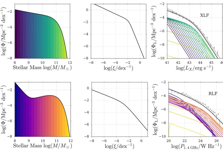
(15) The Astrophysical Journal, 845:134 (33pp), 2017 August 20. Weigel et al.. Figure 6. Summary of our results. We use a simple model to predict the shape of the ERDFs (central panel) for radiatively efficient and inefficient AGNs. We assume that radiatively efficient and inefficient AGNs are predominantly hosted by blue+green and red galaxies, respectively, and thus use these mass function as input for our model. Additionally, we assume that the ERDFs are mass independent and broken power-law shaped and use constant bolometric corrections. The right-hand panels show that, based on these simple assumptions, we are able to predict XLFs and RLFs which are consistent with observations.. quantified the allowed mass dependence of xX (l ) and xR (l ). A mild mass dependence of the ERDFs is consistent with the data and would manifest itself in a mass-dependent AGN fraction. Previous studies have reported AGN fractions that vary as a function of stellar mass (Best et al. 2005; Kauffmann et al. 2008; Hickox et al. 2009; Silverman et al. 2009; Haggard et al. 2010; Xue et al. 2010; Tasse et al. 2011; Janssen et al. 2012; Hernán-Caballero et al. 2014; Williams & Röttgering 2015). However, when interpreting these results it is important to ensure that a possible selection effect has been accounted for.. summarizes mass-independent, but environment-dependent, processes. While environment quenching could, for example, be associated with ram pressure stripping (Gunn & Gott 1972) or strangulation (Larson et al. 1980; Balogh et al. 2000), AGN feedback could be the physical origin of mass quenching. One could imagine a simplistic model in which mass quenching is caused by more AGN activity and thus more AGN feedback at high stellar masses. Massive galaxies could for example be more likely to host AGNs with particularly high Eddington ratios. We have shown that the observations are consistent with a mass-independent xX (l ) model. This is inconsistent with this simplest form of mass quenching. We also discussed models which allow for a mild mass dependence of the ERDF. The linear increase of log l* with log M of up to 1 mag per magnitude in stellar mass is however inconsistent with the exponential increase of the mass quenching probability which the Peng et al. (2010, 2012) model requires. Nonetheless, more sophisticated models could link AGN feedback and mass quenching. For instance, regardless of a massindependent AGN fraction, AGN feedback in low-mass galaxies could be more effective than in high-mass galaxies due to a shallower potential well. Furthermore, AGN feedback might still be a necessary but not sufficient condition for the quenching of star formation. For AGNs with radiatively inefficient accretion, the massindependent ERDF implies that galaxies of all masses are equally likely to host radio AGNs of high and low Eddington. 5.3. AGN Feedback and Quenching AGNs with radiatively efficient and inefficient accretion are thought to play different roles in the quenching of star formation. AGNs with radiatively efficient accretion are considered to be the cause of quenching (Sanders et al. 1988; Di Matteo et al. 2005; Cattaneo et al. 2009; Fabian 2012). AGNs with radiatively inefficient accretion may be keeping their host galaxies quenched (Bower et al. 2006; Croton et al. 2006; Springel et al. 2006; Somerville et al. 2008). In their phenomenological model, Peng et al. (2010, 2012) showed that the stellar mass function of red and quiescent galaxies can be reproduced by splitting the quenching mechanism into two distinct processes. “Mass quenching” is a mass-dependent, but environment-independent, mechanism. “Environment quenching” 15.