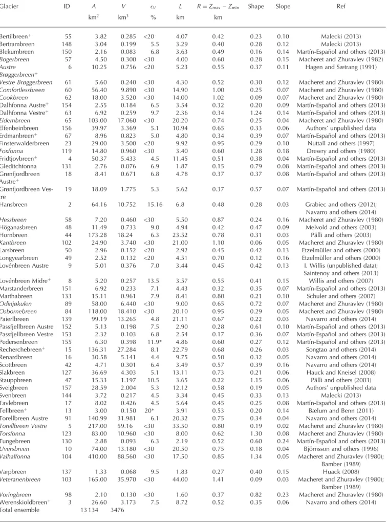
In Table 7,
- the reference for Pedersenbreen should be Songtao and others (2013),
- the reference for Recherchebreen should be Navarro and others (2014).
- the reference for Baalsrudbreen, Blekumnreen, Marstanderbren, and Pasfjellbreen
Vestre and Austre should be Martín-Español (2013),
Estimate of the total volume of Svalbard glaciers, and their
potential contribution to sea-level rise, using new regionally based
scaling relationships
A. MARTÍN-ESPAÑOL,
1F.J. NAVARRO,
1J. OTERO
1, J.J. LAPAZARAN,
1M. BŁASZCZYK
21Department of Applied Mathematics, Universidad Politécnica de Madrid, Madrid, Spain 2Faculty of Earth Sciences, University of Silesia, Sosnowiec, Poland
Correspondence: A. Martín-Español <[email protected]>
ABSTRACT. We present a set of new volume scaling relationships specific to Svalbard glaciers, derived from a sample of 60 volume–area pairs. Glacier volumes are computed from ground-penetrating radar (GPR)-retrieved ice thickness measurements, which have been compiled from different sources for this study. The most precise scaling models, in terms of lowest cross-validation errors, are obtained using a multivariate approach where, in addition to glacier area, glacier length and elevation range are also used as predictors. Using this multivariate scaling approach, together with the Randolph Glacier Inventory V3.2 for Svalbard and Jan Mayen, we obtain a regional volume estimate of 6700835 km3,
or 172 mm of sea-level equivalent (SLE). This result lies in the mid- to low range of recently published estimates, which show values as varied as 13 and 24 mm SLE. We assess the sensitivity of the scaling exponents to glacier characteristics such as size, aspect ratio and average slope, and find that the volume of steep-slope and cirque-type glaciers is not very sensitive to changes in glacier area.
KEYWORDS: Arctic glaciology, volume–area scaling
INTRODUCTION
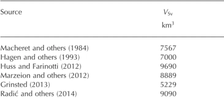
Mass loss from glaciers is currently one of the largest contributors to sea-level rise, with a 27% share of the sum of the total contributions over the period 1993–2010 (Stocker and others, 2013). Moreover, modelling studies show that the contribution to sea-level rise by glaciers will continue to be important during the 21st century. A recent multi-model study suggests a sea-level rise of 15541 mm and 21644 mm over the period 2006–2100, for climate scenarios RCP4.5 and RCP8.5, respectively, involving a reduction of the current global glacier volume by 29% and 41% (Radić and others, 2014). How much and for how long glaciers will continue to be an important contributor to sea-level rise depends on their total volume, the estimate of which has therefore recently received much attention (Radić and Hock, 2010; Huss and Farinotti, 2012; Marzeion and others, 2012; Grinsted, 2013; Radić and others, 2014).
Due to logistic difficulties, glacier volumes determined from ice thickness measurements by methods such as ground-penetrating radar (GPR), seismic soundings or deep ice drilling are available for an extremely small fraction of the total population of glaciers. Adding our 25 glacier volumes reported here to the 337 glacier volumes available in the updated version of the catalogue by Cogley (2012) gives a total of 362 glacier volumes out of a global population of just under 200 000 glaciers in the recent Randolph Glacier Inventory (RGI) V3.2 (Pfeffer and others, 2014), i.e. <0.2%. This small representation highlights the importance of exploring indirect methods to approximate glacier volumes from other known parameters. There are two main indirect methods of inverting for volume from surface properties. Volume–area (V–A) scaling relationships follow from a dimensional analysis of the driving equations of glacier dynamics (Bahr and others, 1997), while
physically based numerical inversion methods are based on numerical inversions relating ice thickness distributions to glacier geometry and dynamics, mass balance and thinning rates (e.g. McNabb and others, 2012). Both methods suffer from the same ill-posed nature of the inversion problem, as all boundary conditions are specified at the glacier surface (Bahr and others, 2014).
Svalbard is a highly glacierized archipelago situated in the Atlantic sector of the Arctic (76–81° N, 10–33° E; Fig. 1), which is a region highly vulnerable to climate change (ACIA, 2005). A recent study by Radić and others (2014), based on multiple climate models, projected mass losses from Svalbard glaciers, over the period 2006–2100, of 12.41 and 15.81 mm sea-level equivalent (SLE) for climate scenarios RCP4.5 and RCP8.5, respectively, representing reductions of 55% and 70% of the current total volume of Svalbard glaciers.
The ice masses of Svalbard cover 33 922 km2 (Pfeffer
and others, 2014), putting this among the largest glacierized areas in the Arctic. The volume of the entire population of Svalbard glaciers has recently been derived, as part of worldwide studies, from global scaling relationships (Mar-zeion and others, 2012; Grinsted, 2013; Radić and others, 2014) and physically based methods as in Huss and Farinotti (2012), revealing high variance across different estimates (Table 1). Older estimates derived from Svalbard-specific scaling relationships (Macheret and Zhuravlev, 1982; Hagen and others, 1993) led to more consistent results. More recent scaling relationships are mostly based on echo sounding flights carried out in the 1970s and 1980s using old radar and positioning systems and mostly consisting of a single profile along the centre line of each glacier (Macheret and Zhuravlev, 1982; Dowdeswell and others, 1984). The corresponding volume estimates, performed assuming para-bolic cross-sections, are expected to have substantial errors. Currently, there is a greater amount of radio-echo sounding data that covers the majority of the surface of the surveyed glaciers. This, combined with improved positioning and recording systems, leads to more accurate volume estimates. In this study we bring together all the available GPR datasets for Svalbard and calculate their associated glacier volumes, which we then use to calibrate new scaling relationships specific to Svalbard glaciers. We then apply these relationships to the most up-to-date glacier inventory, the RGI V3.2 (Pfeffer and others, 2014), to estimate the total volume of Svalbard glaciers and subsequently their total
potential contribution to sea-level rise. Austfonna and Vestfonna are two large ice caps on Nordaustlandet (Fig. 1), which contain much of the glacier volume of Svalbard and have been extensively radio-echo sounded, thus allowing an accurate volume estimate. Since, on the other hand, the number of echo sounded ice caps on Svalbard is insufficient to build a separateV–Arelationship for ice caps, Austfonna and Vestfonna are treated separately, simply adding their GPR-based volume estimates to theV–A
relationship-derived volume estimate for the rest of Svalbard. Jan Mayen is a small (377 km2) island located some
distance (70°560N, 8°320W) from the Svalbard archipelago but is grouped together with it in the RGI. Consequently, we have included its 48 glaciers (covering 120 km2) in ourV–A
relationship-based volume calculations.
DATA
Calibration dataset for the volume–area relationship To derive a reliable volume–area relationship specific to Svalbard glaciers, we need a large sample of accurately measured volume and area pairs, (V,A) pairs, representative of the size distribution of the total population of Svalbard glaciers. The individual glacier volumes are calculated from GPR-retrieved ice thickness data. Therefore, as a first step we compiled, under the framework of the European Science Foundation-supported PolarCLIMATE–SvalGlac project, an inventory of radio-echo sounded glaciers of Svalbard. This inventory is available online at http://svalglac.eu/. There are a total of 314 entries in the inventory, corresponding to 154 different glaciers (many glaciers have been surveyed more than once or have been surveyed using distinct radar equipment). Of these glaciers, we selected only 60 for our sample of (V,A) pairs. The selected sample consists of glaciers for which the net of GPR profiles covers most of the glacier basin and is dense enough to allow for a sufficiently accurate volume estimate.
Our sample of 60 (V,A) pairs was formed as follows. We calculated, from the original GPR ice thickness data, 36 glacier volumes with accuracy in general better than 10%. Of these 36 glaciers, 25 were radio-echo sounded during 1999–2014. Ten of them, located in western Nordenskiöld Land, are reported in Martín-Español and others (2013), and another eight, located in Wedel Jarslberg Land (Fig. 1), are reported in Navarro and others (2014). The remaining seven have not been published elsewhere; five of them are located in western and central Nordenskiöld Land (Fig. 1) and were echo sounded in spring 2013, while two are located in Sabine Land (Fig. 1) and were echo sounded in spring 2014. We also gathered from the literature the ice thickness maps and volumes of six other glaciers with a dense net of GPR profiles and accuracy better than 20% (according to the original sources). This totals 42 glaciers. Our procedure for estimating the error in glacier volume takes into account: (1) the point-dependent ice thickness errors of the GPR data (including the GPS-positioning error, the error in timing and the error in radio-wave velocity), (2) the interpolation error at every gridcell and (3) the volume error stemming from the uncertainty in the glacier boundary delineation. We estimate the interpolation error by using a modified ordinary kriging routine whereby the uncertainty in thickness at a given gridpoint is calculated relating the cross-validation errors with the distance to the nearest GPR measurement. We propagate the data errors to the gridpoints using the same weights adopted in the kriging interpolation procedure. Finally, the errors obtained at each gridpoint are optimally combined and averaged, considering the autocorrelation length scale of the ice thickness, to obtain the volume error. Further details are provided by Martín-Español (2013).
A recent study (Farinotti and Huss, 2013) has shown that, in estimating the accuracy with which the total volume of a glacier population can be recovered from aV–Arelationship,
Table 1.Total volume estimates for Svalbard glaciers (VSv) found in
the literature. All estimates from 2012 onwards use the Randolph Glacier Inventory V2.0, except Marzeion and others (2012), which uses V1.0
Source VSv
km3
the volume measurement uncertainty plays a secondary role compared with the sizes of both the total population and the sample, provided that the latter is sufficiently large. Follow-ing these ideas, we added to our sample some additional entries extracted from the catalogue of glacier volumes of the whole world (Cogley, 2012), reported in Grinsted (2013) (henceforth, referred to as Cogley’s catalogue). Within this catalogue, there are 31 glaciers in Svalbard and 19 of these are different from the 42 so far included in our set of (V,A) pairs. These 19 glaciers correspond to Scott Polar Research Institute–Norsk Polarinstitutt (Dowdeswell and others, 1984) and Soviet (Macheret and Zhuravlev, 1982) airborne radio-echo soundings in the 1970s and 1980s, which only covered the glacier centre lines, but exclude the glaciers with doubtful bed reflection interpretation from Soviet flights discussed by Dowdeswell and others (1984) and later acknowledged by Macheret and others (1984). These glaciers have been used by other authors (e.g. Grinsted, 2013) to build V–A relationships. Of these 19 glaciers we excluded one, Åsgårdfonna, because it is an ensemble of different glacier basins and it is not possible to calculate the volumes of its individual basins. With the addition of these 18 glaciers, for which we assume a volume accurate to better than 30% (Martín-Español, 2013), we obtain our final number of 60 (V,A) pairs.
The basic data for the glaciers in our sample of 60 (V,A) pairs are given in the Appendix, and the location of the glaciers is shown in Figure 1.
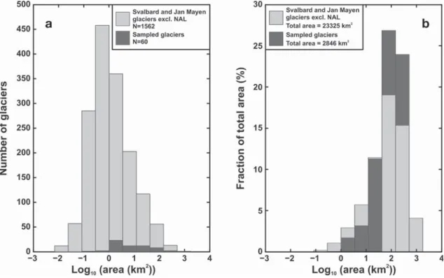
Comparison of the sample with the total population of Svalbard glaciers
The size distribution of our sample dataset ideally should be representative of the total population of Svalbard glaciers. The most up-to-date inventory of Svalbard glaciers is the Randolph Glacier Inventory V3.2 (Pfeffer and others, 2014), which contains the outlines for 1615 individual glacier basins in Svalbard (including Jan Mayen). According to this database, the total glacierized area of Svalbard is 33 922 km2.
This area reduces to 23 325 km2if we exclude Austfonna and
Vestfonna, Nordaustlandet (henceforth referred to asNAL). Figure 2 shows the area distribution of the calibration dataset and compares it with the area distribution of the population of 1562 Svalbard and Jan Mayen glaciers excluding the glacier basins of Nordaustlandet’s ice caps. The RGI contains 300 glaciers (20% of the inventory excludingNAL) larger than 10 km2, which comprise 90% of
the glacier area. The remaining 1261 glaciers (80% of the inventory excludingNAL) are <10 km2and comprise 10% of
the total glacier area. Among the latter, there are 610 glaciers,
glacierets and snowpatches smaller than 1 km2, representing
39% of the inventory and 1% of the total glacier area. In comparison, our sample of 60 glaciers has 31 glaciers (52% of the sample) larger than 10 km2, comprising 95% of the
total sample area, and only 29 glaciers (48% of the sample) equal to or smaller than 10 km2, comprising 5% of the total
area of the sample. Consequently, our sample dataset is biased towards large glaciers. This bias was anticipated, as small valley glaciers are customarily ignored when planning fieldwork because they are often difficult to access and seem less appealing than larger glaciers. To counterbalance this bias towards large glaciers in our sample dataset, we will later introduce an area-related weighting function.
Our calibration dataset is a fair representation of the total population of Svalbard glaciers in terms of terminus type (land-terminating or tidewater): 12 out of 60 glaciers in the sample (20%) are of tidewater type, while 9% of Svalbard glaciers are known to be of tidewater type, but this percentage increases to 14% when glaciers smaller than 1 km2are excluded.
METHODS
We aim to calculate the total volume of Svalbard glaciers using scaling relationships. Volume–area scaling (e.g. Chen and Ohmura, 1990; Bahr and others, 1997) allows esti-mation of the volume of a glacier from its area by means of a power law of the type
V¼cA ð1Þ
where c and are scaling parameters to be calibrated against a given set of (V,A) pairs, which can be done using different techniques, as described below.
We note that the value of derived by Bahr and others (1997), based on dimensional analysis, is= 1.375. Allow-ing slightly differentvalues based on fits to observed data implies moving from a theoretical towards a statistical
approach. This will become clearer later, when we intro-duce the multivariate scaling relations. Nevertheless, we remark that the value derived by Bahr and others (1997) from dimensional analysis is not entirely based on theoret-ical considerations, since it involves closure choices based on observational data. Moreover, the value = 1.375 is based on the assumption of a shallow-ice approximation dynamical model. Considering models slightly differing from it supports the possibility of slightly different values for the exponent in theV–A scaling relationship
Regression techniques
We use two different regression techniques to estimate the parameters c and of the scaling relationships: (1) Least-squares regression in a log-log space (logmse) (Bahr, 1997a):
logmseðpÞ ¼X
n
i¼1
logðVmodelð Þp,i Þ log Vobs,i
2
ð2Þ
where n is the total number of glaciers, Vmodel are the
volumes predicted by the scaling law with a set of param-eters p, and Vobs are the observed volumes in the glacier
volume database. This model is very sensitive to outliers (see, e.g., Grinsted, 2013). (2) Least absolute deviation regression (absdev), proposed by Grinsted (2013), which minimizes the misfit function
absdevðpÞ ¼X
n
i¼1
jVmodelð Þ pffiffiffiffiffiffiffiffiffiffiffi,i Vobs,ij
Aobs,i
p ð3Þ
whereAobs is the observed area of each individual glacier.
As noted by Grinsted (2013), this is a strategy best suited for sea-level rise studies, as it minimizes the absolute volume misfit, in addition to being robust to outliers and asymmetric distributions (Cade and Richards, 1996). This misfit function is weighted by the inverse of the square root of the area, which reduces the sampling bias towards larger glaciers previously identified in our calibration dataset.
Scaling-law parameters for different glacier settings It might be thought a priori that scaling relationships derived for specific types of glaciers would generate better volume predictions than a general-purposeV–Ascaling relationship. However, their expected accuracy improves both with the size of the total target population of glaciers and with the size of the sample used to derive the scaling-law parameters (Farinotti and Huss, 2013). Partitioning a given sample into subgroups by specific characteristics such as glacier size, shape or slope reduces the size of the sample from which the scaling parameters are derived, and hence reduces the expected accuracy in the total volume estimate. Therefore there is a trade-off between the improvement expected by the use of glacier-type specific scaling relationships and the worsening yielded by the reduction of the sample size. We undertook an experiment aimed at verifying whether scaling relationships obtained through characterization of individu-al glacier size or morphology imply significant differences in the estimated volume of Svalbard glaciers, and whether this partitioning implies any noticeable pattern in the scaling exponents, indicative of the influence of particular glacier settings. In particular, we considered partitions of our available sample of Svalbard glaciers by size, shape and slope, as done by Adhikari and Marshall (2012). Shape refers to the horizontal characteristic glacier shape, given by
W=L, where L is the glacier length measured along the central flowline andWis the mean glacier width, defined as
W¼A=L, where A is glacier area. Thus our measure of shape is A=L2. Slope is the mean bedrock slope in the
principal flow direction. As it is not available from measurements done at the glacier surface, following Adhikari and Marshall (2012) we took the mean surface slope, given by E=L, where E is the elevation range, as a proxy of the mean bedrock slope.
Multivariate analysis
Multivariate analysis has proved successful for strengthening the capacity of scaling relationships to estimate glacier volume (Grinsted, 2013). We adopt a multivariate approach to predict the total volume of Svalbard glaciers from a combination of different predictors: glacier area (A), glacier maximum length (L) and glacier elevation range (E). We excluded from this analysis variables such as glacier slope and shape to avoid multicollinearity. We note that, by including additional predictors, we leave the realm of physically based scaling and move towards a statistically based relation. Thus, from statistical tests pursuing the analysis of the variance we found the most significant variables to which to fit the distinct scaling models.
Error estimates
The volume estimates based on V–A scaling relationships can involve very large errors when applied to individual glaciers, though the errors are much lower, because of statistical compensation, when applied to large sets of glaciers. According to Meier and others (2007), estimated volume errors for individual glaciers could exceed 50% but these uncertainties are reduced to 25% for an ensemble of glaciers. Consistent with these results, a recent study by Adhikari and Marshall (2012), using a V–A relationship based on a sample of 280 synthetic random mountain glaciers, has shown that, when estimating the volumes for all individual glaciers in their ensemble, the average glacier volume error is small (2.8%), with a mean absolute error of
18.3%. Their interquartile spread of results is also reason-able, with 50% of errors in the range [–14.7, 15.9]%, but errors for individual glaciers can be high, in the range [–47.6, +99.7]%. Their mean and mean absolute errors for individual glacier volume estimates are reduced to 1.5% and 14.4%, respectively, when shape-based parameters are applied to their random ensemble of glaciers. But these error estimates are too optimistic for a real case in a sense: the sizes of the total population of glaciers to which the scaling relationship is applied and of the calibration dataset from which the scaling parameters are derived are equal, which does not occur in real applications.
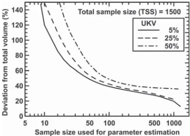
An alternative approach is that of Farinotti and Huss (2013), who have derived upper bound estimates for the accuracy with which the total volume can be recovered in relation to the size of the glacier population, the size of the sample of glaciers used to estimate the scaling parameters and the uncertainty of the measured volumes. Their study has shown that: (1) a low level of accuracy is expected if scaling is applied with coefficients estimated from a small set of samples; (2) accuracy increases with increasing size of the considered glacier population; and (3) volume measurement uncertainty plays a secondary role if a sufficient number of measured glacier volumes are available. The last of these ideas was behind our decision to add to our initial calibration dataset of 42 glaciers, with volume accuracies <20%, 18 additional glaciers with volume accuracies <30%. According to the estimates of Farinotti and Huss (2013), when computing the total volume of 1500 Svalbard glaciers using a V–A relationship based on our sample of 60 measured (V,A) pairs, whose measured volumes have typical accuracies within 5–25%, we could expect a priori an accuracy with an upper bound of 45–50% (Fig. 3). This is an upper bound for the accuracy, and thus a lower bound for the error, derived from synthetic data and only to be reached under ideal conditions (Farinotti and Huss, 2013).
We note, however, that the study by Farinotti and Huss (2013) is based on the assumption of independent and identically distributed (i.i.d.) data pairs. The individual volumes of the global population of glaciers, and the measured volumes and areas, are all assumed to have errors that follow normal (Gaussian) distributions with zero mean
and given standard deviations. These assumptions are violated in our regional study, so there would be no contradiction if our Svalbard-specific scaling law, based on a rather large sample of measured glacier volumes, representative (in terms of spatial distribution and morph-ology) of the total population of Svalbard glaciers, produced better results than those predicted by Farinotti and Huss (2013). We thus adopt an alternative approach, and estimate the error of our total volume calculation following the principles of error propagation (Bevington and Robinson, 2003) and the rationale of Radić and Hock (2010). From the
V–Ascaling model, the total volume is computed as
V¼X
n
i¼1
cAi ð4Þ
The variables and parameters involved in the error inVare thusAi,i¼1,. . .,n,c and, and we assume that they are
random and independent. Then, from error propagation,
V2¼ @V @c
2
c2þ @V @
2
2þXn
i¼1 @V @Ai
2
A2
i ð5Þ
¼ X
n
i¼1 Ai
!2
c2þ X
n
i¼1
cAi logAi
!2 2
þXn
i¼1
cA1
i
2
A2
i ð6Þ
where c, and Ai represent the errors in the
corres-ponding parameters and variables. As typical error in area for Svalbard glaciers we take the value of 8% suggested by König and others (2014). Following the procedure suggested by Bahr (1997b), we estimate the error incas follows. We set a fixed value of (the value obtained for theV–Aregression
retrieved using the 60 glaciers in our sample) and compute 60 individual values forcusing ck¼AVk
k
. We then take as
error incthe standard deviation of the distribution ofck(Fig.
4a), which isc¼0:0109. Likewise, for estimating the error in
we set a fixed value ofc(the value obtained for theV–A
regression retrieved using the 60 glaciers in the sample) and compute 60 individual values for usingk¼ logðlogVkÞðAlogkÞðcÞ.
We then take as error in the standard deviation of the distribution of k (Fig. 4b), which is ¼0:229. Using the
equations and values above, together with the RGI V3.2 for Svalbard (excluding Nordaustlandet ice caps), gives relative errors in the total volume estimate of 767 and 891 km3, when
the logmse and absdev fitting strategies, respectively, are used to derive the V–A relationships. The procedure for estimating the error in the scaling exponent described above differs from the approach taken by Radić and Hock (2010), who approximateby the difference between the value = 1.375 derived theoretically by Bahr and others (1997) and that obtained from theV–Afit to the observations (Bahr, 1997b). Our procedure gives, for the Svalbard case, a larger but more realistic error estimate of(and hence of the volume), and is consistent with the procedure used for estimating the error in the scaling coefficientc.
RESULTS AND DISCUSSION Regression techniques
The results of the calibration of the simpleV–Amodel given by Eqn (1) using our dataset of 60 (V,A) pairs, by means of bothlogmseandabsdev regression techniques, are shown in Table 2 and Figure 5. Table 2 also includes the cross-validation error based on the calibration dataset, estimated by leave-one-out cross-validation (Geisser, 1993), and the coefficient of determinationR2 of the fit, and also presents
the volumes computed by each scaling relationship and their estimated errors, calculated as described in the previous subsection. The absolute errors in volume shown in Table 2 correspond to relative errors of 20% (logmse) and 24% (absdev), and the volume estimates differ from each other by5%.
Cross-validation is estimated as follows. In k-fold cross-validation, the original sample is randomly partitioned intok
equal-size subsamples. Of the k subsamples, a single subsample is retained as the validation data for testing the model, and the remaining k-1 subsamples are used as training data. The cross-validation process is then repeated
Fig. 4.Histograms of the distributions for parameters andc.
Table 2. Derived scaling law and associated total volume of Svalbard glaciers (excludingNAL) calculated using thelogmseand
absdev regression techniques. The cross-validation error crossval
and the coefficient of determinationR2are also given.
Strategy Scaling law crossval
RMSE
R2 Svalbard vol.
excl.NAL
km3
logmse 0.0343A1:329 6.02 0.98 3955767
ktimes, with each of theksubsamples used exactly once as validation data. Leave-one-out cross-validation is the same as ak-fold cross-validation withkbeing equal to the number of observations in the original sample. In each case, all observations are used for both training and validation, and each observation is used for validation exactly once. The cross-validation errors shown in Table 2 are the root-mean-square errors (RMSE) for the volumes estimated during the leave-one-out cross-validation procedure.
To verify that our derived scaling relationships are not influenced by the original bias in the size distribution of the glacier sample, we performed, for each of the regression techniques, the following test. For each particular glacier in our sample, we computed the residual volume obtained by subtracting, from the volume of the glacier computed from GPR data, the estimated volume of that particular glacier derived from aV–A scaling law obtained by removing that particular glacier from the sample. We then plotted the residual volume versus the area of the glacier. No significant correlation was found, indicating that there is no noticeable influence of the original bias in the size distribution of the glacier sample on our derived scaling relationships.
Scaling-law parameters for different glacier settings The results for the best-fitting scaling parameterscandfor specific subgroups of glaciers arranged by size, shape and slope, using both thelogmse and absdev fitting strategies, are shown in Table 3. Overall, partitioning by size yields poorer fits and the smallest volume for the entire population of Svalbard glaciers excludingNAL(V ½3561, 3656km3),
whereas the largest correspond to the partitionings by shape (V ½3867, 3897km3) and slope (V ½3579, 4144km3).
We also calculate for a constrained value of c¼
0:0343, taken from the logmse regression for the entire population of glaciers (Table 2). Here we use the logmse
misfit function rather than the absdev approach because
logmseis most often used in the literature and provides a value forccloser to those obtained by other authors, which facilitates comparison of the values. The results of the
constrained experiment show minimum values for the highest ranges of slope and shape, in agreement with the results obtained by Adhikari and Marshall (2012) for a collection of synthetic glaciers. This means that the volumes of steep-slope and cirque-type glaciers are less sensitive to changes in glacier area. This could actually be an indication that response timescales play a role. In particular, long, steep glaciers presumably have a different response time than short, flat glaciers, which means that current disequilibrium between volume and shape, caused by the ongoing mass losses, expresses itself in different optimal parameter values. Recalling, from Table 2, that the total volume of Svalbard glaciers excludingNAL, computed using a single scaling law for all glaciers and thelogmsemisfit function, was 3955 km3,
we see that the constrained experiment gives volumes that are2% smaller when using partitionings by size or shape, while nearly equal (only slightly larger) when using partitioning by slope. We note, however, the small number of glaciers belonging to some of the subgroups, which
Table 3.Scaling-law parameters for different glaciological settings (following Adhikari and Marshall (2012), adapting ranges to our sample distribution). In addition to thelogmseandabsdevfitting strategies, results are also presented for a constrained experiment in which a fixed value ofcis used (c¼0:0343) and onlyis fit. The coefficients of determinationR2of the different regressions are given, as well as the total
volume of Svalbard glaciersVSv(excludingNAL) calculated using the given partitions into subgroups of glaciers. Values in brackets indicate
the number of glaciers in each subgroup
Class A Class B Class C Total volume
c R2 c R2 c R2 V
Sv
km3
Size,A(km2) 10 [29] 10–100 [22] 100 [9]
logmse 0.0379 1.225 0.88 0.0356 1.336 0.89 0.131 1.067 0.76 3561
constrained – 1.286 0.98 – 1.346 0.99 – 1.321 0.99 3886
absdev 0.0379 1.251 0.84 0.0408 1.303 0.89 0.1121 1.099 0.81 3656
Shape,W=L 0.3 [27] 0.3–0.5 [20] 0.5 [13]
logmse 0.0384 1.335 0.99 0.0347 1.307 0.97 0.0282 1.326 0.99 3867
constrained – 1.365 0.99 – 1.310 0.99 – 1.275 0.97 3894
absdev 0.0375 1.345 0.99 0.0377 1.289 0.88 0.0378 1.266 0.99 3897
Slope,E=L 0.05 [13] 0.05–0.1 [25] 0.1 [22]
logmse 0.0251 1.394 0.92 0.0330 1.347 0.95 0.0390 1.223 0.93 4144
constrained – 1.329 0.99 – 1.335 0.99 – 1.297 0.98 3969
absdev 0.0948 1.137 0.92 0.0676 1.152 0.98 0.0477 1.115 0.93 3579
Fig. 5.Volume–area scaling models calibrated using the logmse
probably lie near the minimum admissible number for reaching statistically significant conclusions.
In our study of Svalbard glaciers, a straightforward partitioning would be to distinguish between tidewater and land-terminating glaciers. However, for our sample of (V,A) pairs this partitioning is nearly equivalent to a partitioning by size (with the tidewater glaciers being the largest), so it gives no further insight. Another clear classification criterion would be a grouping into surging and non-surging glaciers. In this case, the available set of (V,A) pairs for surging glaciers is so small that it does not allow us to derive a specific scaling law. Moreover, the volume–area ratios of surging glaciers are dependent upon the surge phase: while during the early post-surge period surging glaciers will generally have smaller volume–area ratios than non-surging glaciers, during the build-up period of the surge the converse will generally be true. As a sensitivity test, we removed the surge glaciers from our calibration dataset and, keeping c
fixed, we recalculated the value of the exponent . This resulted in a slightly larger scaling exponent,= 1.333 (using thelogmsefitting strategy), which indicates that most of the surge glaciers included in our sample are in their early post-surge period, with a consequently smaller volume–area ratio.
Multivariate analysis
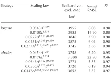
A multivariate statistical analysis reveals that a simple model
V/A in the log-log space explains 98.6% of the variance. However, the analysis of the cross-validation errors reveals that results are improved when all the variables are included in the model, i.e.V¼cA1L2E3, especially for thelogmse misfit function, as more significant glaciological information is used to predict glacier volume. Table 4 shows the ice volume estimates for Svalbard using different regression models, and their accuracy, estimated in terms of leave-one-out cross-validation errors. Accuracy is strongly reduced in the models where the variableAis not present (14.9% and 22.9% cross-validation RMSE), in contrast to the results obtained by Radić and others (2008), whereV/L had the lowest error. In general thelogmsestrategy provides lower cross-validation errors, the lowest corresponding to the
V¼cA1L2E3 scaling law, although the small exponent of
E (Table 4) confirms the low predicting capability of this variable.
Comparison with otherV–A scaling relationships In Table 5 we compare our results for the glacier volume of Svalbard excluding Nordaustlandet (VSvexcl:NAL) with those obtained using other scaling relationships available in the literature. For the sake of homogeneity, the RGI V3.2 is used for all of them, and we use our standardV–A scaling law (instead of the multivariate), as most published relationships are of theV–Atype. Also for this reason we choose, among the distinct relationships presented by Grinsted (2013) (several of them multivariate), his standard V–A scaling law. All scaling relationships included in the table are of the
V–A type, except those of Hagen and others (1993) and Huss and Farinotti (2012), which are of theH–A type, with
Hthe mean glacier thickness. Because of this, the exponent
in Huss and Farinotti’s relationship is nearly 1 unit lower than those for the univariateV–Arelationships, and also the coefficientcis substantially different. As a complementary test of performance, we also present the percentage of error incurred when calculating the total volume of our cali-bration dataset using the relationships from other published scaling models (Table 5; we exclude ours, since their results would be skewed). The estimates in Table 5 range within 2462–6170 km3, with an average value of 44211037 km3
if we exclude our own estimates, and 4334971 km3if our
results are included. In both cases, the quoted errors indicate the standard deviations of the different estimates considered, which illustrates the spread of the results.
In addition to the scaling relationships derived in this study, those by Macheret and others (1984) and Hagen and
Table 5. Total volume estimates for Svalbard glaciers (VSv),
excluding NAL, calculated using various scaling relationships found in the literature, together with our own, and relative errors produced when these scaling laws are applied to our calibration dataset (VSample). Note that the values of the coefficientcin theV–A
scaling laws are given in km32, withthe exponent of the scaling
law, while in the literature they are often given in m32
Source Scaling law VSvðexcl:NALÞ VSample*
km3 %
This study,logmse V¼0:0343A1:329 3955 n/a
This study,absdev V¼0:0454A1:264 3758 n/a
Macheret and others (1984) V¼0:0371A1:357 4957 31.9
Hagen and others (1993)y H¼33 lnðAÞ þ25
ifA>1 km2 4042 8.92 H¼25 ifA<1 km2
Chen and Ohmura (1990) V¼0:0285A1:357 3808 1.34
Bahr and others (1997) V¼0:0276A1:36 3746 –0.3
Huss and Farinotti (2012)y H¼0:310A0:355 4099 47.2
Adhikari and Marshall (2012) V¼0:027A1:458 6170 62.9
Shape – Glaciers 4260 –13.6 Slope – Glaciers 2462 25.3
Size – Glacier 5633 50.7 Grinsted (2013) V¼0:0433A1:29 4090 8.9
Radić and others (2014) V¼0:0365A1:375 5360 42.5
*VSampleis calculated asððVmodeliVsampleÞ=VsampleÞ 100. Not shown for our
scaling relationships to avoid biased results.
yHis the mean ice thickness (m).Ashould be given in km2. The units of the
coefficient in the Huss and Farinotti relationship are 103km12.
Table 4.Scaling laws resulting from the multivariate analysis, and their associated estimates of the total volume of Svalbard (excluding
NAL), together with the cross-validation errors incurred when calculating the total volume of the 60 glaciers in our calibration dataset using these scaling laws, and the corresponding coefficients of determinationR2
Strategy Scaling law Svalbard vol. excl.NAL
crossval
RMSE
R2
km3
logmse 0.0343A1:329 3955 6.08 0.98
0.0150L2:333 3955 14.90 0.88
0.0272A1:113L0:429 3846 3.90 0.98
0.0451A1:283E0:239 3875 6.02 0.98
0.0277A1:115L0:423E0:012 3745 3.86 0.98
absdev 0.0454A1:264 3758 6.20 0.95
0.0176L2:331 3,388 22.90 0.46
0.0343A1:162L0:270 3773 5.55 0.97
0.0586A1:228E0:403 3728 6.19 0.94
others (1993) are specific to Svalbard glaciers. However, those two studies were based on a glacier inventory of Svalbard several decades older than ours, so their areas and volumes are generally larger due to the overall retreating and thinning trends of Svalbard glaciers during recent decades (Nuth and others, 2007, 2010). As shown in Table 5, the scaling approach of Macheret and others (1984) overestimates the total volume of the calibration dataset by 32%, while that of Hagen and others (1993) also over-estimates it, but only by 9%. This could be an indication that the volume–area relationship of Svalbard glaciers has varied over the past 30 years, with mass loss dominated by glacier thinning rather than front retreat, which is consistent with observations (e.g. Nuth and others, 2007, 2010), resulting in smallerV=Aratios. But these results could also partly reflect some bias in the glacier volume data used to derive the mentioned scaling relationships.
By far the closest estimates to both our results for the total volume of Svalbard glaciers (excludingNAL) and the total volume of the calibration dataset are those obtained using the scaling relationships of Chen and Ohmura (1990) and Bahr (1997a). These scaling approaches are based on a global sample of valley glaciers. We might think that, having excluded Austfonna and Vestfonna, the calibration datasets of both these global relationships and our regionally based one are somehow similar. However, the good fit is still surprising considering the large proportion of tidewater glaciers within the sample of Svalbard glaciers compared with the samples by Chen and Ohmura (1990) and Bahr (1997b). The scaling approaches of Huss and Farinotti (2012) and Grinsted (2013) also provide total volume estimates close to our own. However, when estimating the volume of the calibration dataset, the relationship by Huss and Farinotti (2012), which is a regional scaling law derived from the entire set of Svalbard glacier volumes computed with the physically based method developed by those authors, gives a large overestimate of 47%. A possible explanation is that, being a scaling relation based on the complete set of volumes, it gives a good approach to the volume of the total population, while, when applied to our sample, it does not provide such a good fit because the sample is not fully representative of the size distribution of the complete population of Svalbard glaciers.
The largest estimates of the total volume of Svalbard excluding NAL are those obtained using the scaling by Adhikari and Marshall (2012), derived from their entire set of synthetic glaciers (without any partitioning by glacier types), and that based on partitioning by size. These also produce the largest overestimates of the volume of the calibration dataset. By contrast, the relationship based on partitioning by slope gives by far the lowest total volume estimate (but overestimates the volume of the sample), while that based on partitioning by shape produces a mid- to high total volume estimate (but underestimates the volume of the sample). Table 5 shows that, in general, a high total volume estimate is accompanied by an overestimate of the volume of the sample, and conversely. The scalings of Adhikari and Marshall (2012) based on partitionings by slope and shape are an exception to this rule. The most likely reason is the irregular distribution of glaciers in our sample among the three slope and shape ranges considered by Adhikari and Marshall (2012), 50–10–0 (slope) and 16–35–9 (shape), while the distribution is more regular in the case of partitioning by size (26–10–24). We note that the ranges of
the partitionings by size, shape and slope in our experiment in the subsection ‘Scaling-law parameters for different glacier settings’ above, and in Adhikari and Marshall (2012) are different. This is why our experiment using partitioning (which had a fair distribution of glaciers among the different ranges of variation of a given attribute) produced good results (consistent with the experiments without partitioning), while Adhikari and Marshall (2012) also produced good results when working with their sample of glaciers (which also had a fair distribution of glaciers among the different ranges of each partitioning), but not when applied to our population and sample of Svalbard glaciers. From this we conclude that the scaling relationships based on partitionings by glacier attributes such as size, shape or slope are expected to produce good results provided the size of the sample is large enough and has a fair distribution of glaciers among the different ranges of values of each attribute, which should also be representative of the distribution existing in the total glacier population. While this representativeness calls for regionally based relationships, the main difficulty faced in this case is the requirement of a large sample. Our Svalbard partitioning experiment seems to be near the minimum admissible number of sampled glaciers.
The total volume estimate obtained using the scaling by Radić and others (2014) is also large, and their relationship greatly overestimates (by 43%) the volume of the calibration dataset. This illustrates how sensitive are the volume calculations from volume–area relationships to the choice of the scaling parameters, since Radić and others (2014) adopt a scaling law that uses theccoefficient obtained by Chen and Ohmura (1990) (which produced results close to ours when used with its own exponent¼1:357) together with the exponent¼1:375 derived by Bahr and others (1997) based on physical considerations for mountain glaciers (which we note is different from the ¼1:36 obtained by Bahr (1997a) that gave results close to ours when used with its associated c coefficient). It should be noted that theccoefficients in theV–Ascaling laws in Table 5 are given in units of km32 and therefore depend on the choice of . Since the fits for c and are obtained simultaneously, and the parameter values are therefore mutually influenced, we do not recommend taking separate values forcandfrom independent studies. If a value is taken from a theoretical study, as done by Radić and others (2014) following Radić and Hock (2010), then the c
coefficient should ideally be obtained from a fit to measured volumes (keeping fixed the selected exponent).
Total volume of Svalbard glaciers and potential contribution to sea-level rise
Our best estimates of the total volume of Svalbard glaciers, excluding Austfonna and Vestfonna, are those given by our multivariate scaling relationships including the glacier area, length and altitude range as variables. The results obtained using the logmse and absdev regression techniques, extracted from Table 4, are given in Table 6 accompanied by their error estimates calculated as described in the ‘Error estimates’ subsection above. To obtain the total volume of Svalbard glaciers we simply add the volumes of Austfonna and Vestfonna determined from extensive radio-echo sounding (both airborne and surface-based) as described by Dunse (2011), Pettersson and others (2011) and Martín-Español (2013), which are 2559 km3 (Austfonna) and
and 7%, estimated by Martín-Español (2013). Thus, the ice volume of Nordaustlandet ice caps totals 300181 km3.
The resulting total volume of Svalbard glaciers is given in Table 6, where the errors from scaling (Svalbard excluding
NAL) and GPR (NAL) are combined as the square root of the sum of squares. The values based on both regression techniques are shown, and we can consider their average, 6700835 km3, as our best estimate of Svalbard ice
volume. In terms of sea-level equivalent (SLE), assuming an oceanic area of 3:62108km2and a glacier ice density
of 900 kg m3, our volume estimate corresponds to a total
potential contribution to sea-level rise of 172 mm SLE. This volume estimate is in the low range of those published in the literature (Table 1), including the regionally based estimates of Macheret and others (1984) and Hagen and others (1993), but higher than that of Grinsted (2013). We note that the volumes given in Table 1 are based on different inventories. This should have an impact especially on the estimates by Macheret and others (1984) and Hagen and others (1993). The most recent estimates (including ours) are all based on the RGI. Although the RGI version used sometimes differs, this should have little impact on the results. Although the number of glacier complexes world-wide is different in RGI V1.0 and V2.0 compared with V3.2 (Pfeffer and others, 2014), and this could have an impact on the volume calculations, the number of glacier complexes in the particular case of Svalbard has not changed between RGI versions (Arendt and others, 2014). The only change from V1.0 to V2.0 that has an impact on glacier volume is that the outlines of Jan Mayen were included. This implies an increase in volume of8–9 km3(depending on the scaling
relation used), which only applies to the comparison between the estimate by Marzeion and others (2012), based on RGI V1.0, and all later ones, based on V2.0 except ours, based on V3.2. We also recall that all results except that of Huss and Farinotti (2012) (derived from a physically based method) are based on scaling relationships, and that our estimate combines scaling (for Svalbard excluding Nordaust-landet) and direct calculation from GPR-retrieved ice-thickness data (for Nordaustlandet ice caps). We also note that, in all versions of the RGI, Austfonna and Vestfonna (and also ice caps covering other islands of the Svalbard archipelago) appear subdivided into individual drainage basins, and that currently theRGIflagattribute of the RGI only distinguishes between glaciers and ice caps for the Antarctic and Subantarctic RGI region (Pfeffer and others, 2014). Consequently, any scaling-based estimate, even if it has separate scaling laws for glaciers and ice caps, if applied to Svalbard (or any region other than the Antarctic and Subant-arctic) using the RGI without corrections, will compute the
volume of each entry in the inventory as if it were a glacier. This will likely lead to biased results. With the aim of quantifying the differences for the case of Austfonna and Vestfonna, we calculated their volumes as the sum of the volumes of all their basins, as defined in the RGI V3.2, using ourV-Ascaling (as done, e.g., by Grinsted, 2013). This gives a total volume of Nordaustlandet ice caps of 2444 km3
(averaging thelogmse- andabsdev-based results), which is 557 km3lower than the volume of 3001 km3obtained from
the GPR data. Nearly all the difference (546 km3)
corres-ponds to Austfonna. Using the scaling-based estimate for all of Svalbard gives a total volume of 6143 km3, making our
result closer to that of Grinsted (2013). It would be even closer (6003 km3) if we took ourabsdev-based result (recall
that Grinsted’s result is also based on theabsdevregression). We stress, anyway, that the GPR-based volume estimate for Austfonna and Vestfonna is more credible than any estimate based on scaling relationships.
SUMMARIZING CONCLUSIONS
Using 60 highly accurate Svalbard volume–area pairs, with volumes calculated from GPR data, we calibrated different scaling relationships with the aim of estimating the total volume of Svalbard glaciers and, thus, their potential contribution to sea-level rise. These relationships were applied to each glacier record included in the RGI V3.2 for Svalbard and Jan Mayen. We estimated the total ice volume of Svalbard glaciers at 6700835 km3, or 172 mm SLE.
We obtained evidence, from the slope- and shape-based scaling relationships, that the volumes of steep-slope and cirque-type glaciers appear to be less sensitive to changes in glacier area. An alternative interpretation is that they could just have different response times. The multivariate analysis shows minimum cross-validation errors when the volume– area–length–elevation range scaling model is used, for both the logmse and absdev regression techniques, which suggests that the use of multivariate scaling relationships improves the accuracy as compared with the standard volume–area scalings. Our estimate of the Svalbard glacier volume lies in the low range of previously published estimates, with only the estimate by Grinsted (2013) providing a lower volume. However, a fair comparison is difficult, as the published estimates are based on different inventories. Fortunately, the most recent estimates are all based on the RGI, and, even if based on different versions of it, the only difference corresponds to the 8–9 km3of added
volume corresponding to the Jan Mayen glaciers from RGI V2.0 onwards. An additional difficulty is that not all scaling relations are of the V–A type, but some include further variables. Also, the way of dealing with Austfonna and Vestfonna ice caps, which appear in the RGI subdivided into individual basins, all classified as glaciers, could make a difference. For this reason, we made a comparison based on the use of the RGI V3.2 for all scaling relationships, and restricted to Svalbard glaciers excluding Austfonna and Vestfonna. This comparison showed that globally based relationships sometimes provide results close to regionally based ones. Their suitability, rather than depending on being globally or regionally based, depends on how well the sample of glaciers from which the scaling relationship is derived represents the actual distribution of the total population of glaciers of the region under study. Of course other factors, such as the sample size, the total population
Table 6.Estimated total glacier volume of Svalbard and its potential contribution to sea-level rise
Regression VSvNAL(scaling) VNAL(GPR) Total volume SLE*
km3 km3 km3 mm
logmse 3745767 300181 6746771 172
absdev 3652891 300181 6653895 172
Average 6700835 172 *Sea level is calculated assuming an oceanic area of 3:62108km2and a
size and the accuracy of the individual volumes in the sample, also play an important role, as shown by Farinotti and Huss (2013). Regarding this, our calibration dataset of 60 (V,A) pairs, with volume errors typically within 5–25% but quite often <10%, and being a fair representation of the size distribution of the total population of Svalbard glaciers, strongly supports the accuracy of our estimate in comparison with other published estimates. The accuracy of our estimate is also expected to have been improved by the use, for Austfonna and Vestfonna, of the volume calculated directly from the GPR-retrieved ice-thickness data. The comparison also demonstrated the sensitivity of the volume estimates to the scaling parameters and, in particular, that the coefficient
cand the exponentshould be fitted simultaneously. More specifically, if one of these is taken from theoretical considerations, the other should be fitted against available volume measurements rather than taking it from other fits available in the literature. Finally, a note of caution is sounded about the use of the RGI together with scaling relationships distinguishing between glaciers and ice caps, since none of the currently available RGI versions identifies the ice caps (i.e. all inventory entries appear as glacier), except for the Antarctic and Subantartic RGI regions. This calls for the completion of this important attribute in the RGI.
ACKNOWLEDGEMENTS
This research was supported by grant EUI2009-04096 (PolarCLIMATE-SvalGlac) from the Spanish EuroResearch Programme, grants CGL2005-05483, CTM2008-05878 and CTM2011-28980 from the Spanish National Plan for R&D, grant NCBiR/PolarCLIMATE-2009/2-2/2010 from the Polish National Centre for R&D, grants IPY/269/2006 and N N306 094939 from the Polish Ministry of Science and Higher Education, Polish–Norwegian funding through the AWAKE (PNRF-22-AI-1/07) project, and grants 10-05-00133-a and 11-05-00728-a from the Russian Fund of Basic Research. We are grateful for the suggestions by Graham Cogley, Surendra Adhikari, Ben Marzeion and an anonymous reviewer, as well as the work of the scientific editor, Jo Jacka, which greatly improved the manuscript.
REFERENCES
Adhikari S and Marshall SJ (2012) Glacier volume–area relation for high-order mechanics and transient glacier states. Geophys. Res. Lett.,39(16), L16505 (doi: 10.1029/2012GL052712) Arctic Climate Impact Assessment (ACIA) (2005) Arctic Climate
Impact Assessment: scientific report. Cambridge University Press, Cambridge
Arendt A and 81 others (2014)Randolph Glacier Inventory (RGI), Vers. 4.0: a dataset of global glacier outlines.Global Land Ice Measurements from Space, Boulder, CO. Digital media: http:// www.glims.org/RGI/
Bælum K and Benn DI (2011) Thermal structure and drainage system of a small valley glacier (Tellbreen, Svalbard), investi-gated by ground penetrating radar.Cryosphere,5(1), 139–149 (doi: 10.5194/tc-5-139-2011)
Bahr DB (1997a) Width and length scaling of glaciers.J. Glaciol.,
43(145), 557–562
Bahr DB (1997b) Global distributions of glacier properties: a stochastic scaling paradigm. Water Resour. Res., 33(7), 1669–1679 (doi: 10.1029/97WR00824)
Bahr DB, Meier MF and Peckham SD (1997) The physical basis of glacier volume–area scaling. J. Geophys. Res., 102(B9), 20 355–20 362 (doi: 10.1029/97JB01696)
Bahr DB, Pfeffer WT and Kaser G (2014) Glacier volume estimation as an ill-posed inversion. J. Glaciol., 60(223), 922–934 (doi: 10.3189/2014JoG14J062)
Bamber JL (1989) Ice/bed interface and englacial properties of Svalbard ice masses deduced from airborne radio echo-sounding data. J. Glaciol., 35(119), 30–37 (doi: 10.3189/ 002214389793701392)
Bevington PR and Robinson DK (2003)Data reduction and error analysis for the physical sciences, 3rd edn. McGraw-Hill, New York
Björnsson H and 6 others (1996) The thermal regime of sub-polar glaciers mapped by multi-frequency radio-echo sounding.
J. Glaciol.,42(140), 23–32
Cade BS and Richards JD (1996) Permutation tests for least absolute deviation regression.Biometrics,52(3), 886–902
Chen J and Ohmura A (1990) Estimation of Alpine glacier water resources and their change since the 1870s. IAHS Publ. 193 (Symposium at Lausanne 1990 – Hydrology in Mountainous Regions), 127–135
Cogley JG (2012) The future of the world’s glaciers. In Henderson-Sellers A and McGuffie K eds. The future of the world’s climate. Elsevier, Waltham, MA, 197–222
Dowdeswell JA, Drewry DJ, Liestøl O and Orheim O (1984) Radio echo-sounding of Spitsbergen glaciers: problems in the inter-pretation of layer and bottom returns.J. Glaciol.,30(104), 16–21 Drewry DJ, Liestøl O, Neal CS, Orheim O and Wold B (1980) Airborne radio echo sounding of glaciers in Svalbard. Polar Rec.,20(126), 261–266
Dunse T (2011) Glacier dynamics and subsurface classification of Austfonna, Svalbard: inferences from observations and model-ling. (PhD thesis, University of Oslo)
Etzelmüller B, Ödegård RS, Vatne G, Mysterud RS, Tonning T and Sollid JL (2000) Glacier characteristics and sediment transfer system of Longyearbreen and Larsbreen, western Spitsbergen.
Nor. Geogr. Tidsskr.,54(4), 157–168
Farinotti D, Huss M, Bauder A and Funk M (2009) An estimate of the glacier ice volume in the Swiss Alps.Global Planet. Change,
68(3), 225–231 (doi: 10.1016/j.gloplacha.2009.05.004) Farinotti D and Huss M (2013) An upper-bound estimate for the
accuracy of glacier volume–area scaling. Cryosphere, 7(6), 1707–1720 (doi: 10.5194/tc-7-1707-2013)
Frey H and 9 others (2013) Ice volume estimates for the Himalaya– Karakoram region: evaluating different methods. Cryos. Dis-cuss.,7(5), 4813–4854 (doi: 10.5194/tcd-7-4813-2013) Geisser S (1993) Predictive inference: an introduction.
(Mono-graphs on Statistics & Applied Probability 53) Chapman & Hall, New York
Grabiec M, Jania J, Puczko D, Kolondra L and Budzik T (2012) Surface and bed morphology of Hansbreen, a tidewater glacier in Spitsbergen.Pol. Polar Res.,33(2), 111–138 (doi: 10.2478/ v10183-012-0010-7)
Grinsted A (2013) An estimate of global glacier volume. Cryo-sphere,7(1), 141–151 (doi: 10.5194/tc-7-141-2013)
Hagen JO and Sætrang A (1991) Radio-echo soundings of sub-polar glaciers with low-frequency radar.Polar Res.,9(1), 99–107 (doi: 10.1111/j.1751-8369.1991.tb00405.x)
Hagen JO, Liestøl O, Roland E and Jørgensen T (1993) Glacier atlas of Svalbard and Jan Mayen.Nor. Polarinst. Medd.129 Hauck C and Kneisel C (2008)Applied geophysics in periglacial
environments.Cambridge University Press, Cambridge Huss M and Farinotti D (2012) Distributed ice thickness and
volume of all glaciers around the globe. J. Geophys. Res.,
117(F4), F04010 (doi: 10.1029/2012JF002523)
Huss M and Farinotti D (2014) A high-resolution bedrock map for the Antarctic Peninsula.Cryosphere,8(4), 1261–1273 (doi: 10.5194/ tc-8-1261-2014)
Lapazaran J and 6 others (2013) Ice volume changes (1936–1990– 2007) and ground-penetrating radar studies of Ariebreen, Hornsund, Spitsbergen. Polar Res.,32, 11068 (doi: 10.3402/ polar.v32i0.11068)
Macheret Y and Zhuravlev AB (1980) Radiolokatsionnoye zondir-ovaniye lednikov Shpitsbergena s vertoleta [Radio echo-sound-ing of Spitsbergen’s glaciers from a helicopter].Mater. Glyatsiol. Issled./Data Glaciol. Stud.,37, 109–131 [in Russian with English summary]
Macheret YuYa and Zhuravlev AB (1982) Radio echo-sounding of Svalbard glaciers.J. Glaciol.,28(99), 295–314
Macheret Y, Zhuravlev AB and Bobrova LI (1984) Tolshchina, podlednyy rel’yef i ob’’yem lednikov Shpitsbergena po dannym radiozondirovan-iya [Thickness, subglacial relief and volume of Svalbard glaciers from radio echo-sounding data]. Mater. Glyatsiol. Issled.,51, 49–63 [in Russian with English summary] Malecki J (2013) The actual state of Svenbreen (Svalbard) and changes of its physical properties after the termination of Little Ice Age. (PhD thesis, Adam Mickiewicz University)
Martín-Español A (2013) Estimate of the total ice volume of Svalbard glaciers and their potential contribution to sea-level rise. (PhD thesis, Polytechnic University of Madrid)
Martín-Español and 7 others (2013) Radio-echo sounding and ice volume estimates of western Nordenskiöld Land glaciers, Svalbard. Ann. Glaciol., 54(64), 211–217 (doi: 10.3189/ 2013AoG64A109)
Marzeion B, Jarosch AH and Hofer M (2012) Past and future sea-level change from the surface mass balance of glaciers.
Cryosphere,6(6), 1295–1322 (doi: 10.5194/tc-6-1295-2012) McNabb RW and 11 others (2012) Using surface velocities to
calculate ice thickness and bed topography: a case study at Columbia Glacier, Alaska, USA.J. Glaciol.,58(212), 1151–1164 (doi: 10.3189/2012JoG11J249)
Meier MF and 7 others (2007) Glaciers dominate eustatic sea-level rise in the 21st century.Science,317(5841), 1064–1067 (doi: 10.1126/science.1143906)
Melvold K, Schuler T and Lappegard G (2003) Ground-water intrusions in a mine beneath Høganesbreen, Svalbard: assessing the possibility of evacuating water subglacially.Ann. Glaciol.,
37, 269–274 (doi: 10.3189/172756403781816040)
Navarro FJ and 6 others (2014) Ice volume estimates from ground-penetrating radar surveys, Wedel Jarlsberg land glaciers, Svalbard.Arct. Antarct. Alp. Res.,46(2), 394–406
Nuth C, Kohler J, Aas HF, Brandt O and Hagen JO (2007) Glacier geometry and elevation changes on Svalbard (1936–90): a baseline dataset. Ann. Glaciol., 46, 106–116 (doi: 10.3189/ 172756407782871440)
Nuth C, Moholdt G, Kohler J, Hagen JO and Kääb A (2010) Svalbard glacier elevation changes and contribution to sea level rise.
J. Geophys. Res.,115(F1), F01008 (doi: 10.1029/2008JF001223) Nuttall A-M, Hagen JO and Dowdeswell J (1997) Quiescent-phase changes in velocity and geometry of Finsterwalderbreen, a surge-type glacier in Svalbard.Ann. Glaciol.,24, 249–254 Pälli A, Moore JC, Jania J and Głowacki P (2003) Glacier changes in
southern Spitsbergen, Svalbard, 1901–2000.Ann. Glaciol.,37, 219–225 (doi: 10.3189/172756403781815573)
Pettersson R, Christoffersen P, Dowdeswell JA, Pohjola VA, Hubbard A and Strozzi T (2011) Ice thickness and basal conditions of Vestfonna Ice Cap, eastern Svalbard.Geogr. Ann. A,93(4), 311–322 (doi: 10.1111/j.1468-0459.2011.00438.x) Pfeffer WT and 19 others (2014) The Randolph Glacier Inventory: a
globally complete inventory of glaciers. J. Glaciol., 60(221), 537–552 (doi: 10.3189/2014JoG13J176)
Radić V and Hock R (2010) Regional and global volumes of glaciers derived from statistical upscaling of glacier inventory data.
J. Geophys. Res.,115(F1), F01010 (doi: 10.1029/2009JF001373) Radić V, Hock R and Oerlemans J (2008) Analysis of scaling methods in deriving future volume evolutions of valley glaciers.J. Glaciol.,
54(187), 601–612 (doi: 10.3189/002214308786570809) Radić V, Bliss A, Beedlow AC, Hock R, Miles E and Cogley JG
(2014) Regional and global projections of twenty-first century glacier mass changes in response to climate scenarios from global climate models. Climate Dyn., 42(1–2), 37–58 (doi: 10.1007/s00382-013-1719-7)
Saintenoy A and 7 others (2013) Deriving ice thickness, glacier volume and bedrock morphology of Austre Lovénbreen (Svalbard) using GPR. Near Surf. Geophys., 11(2), 253–261 (doi: 10.3997/1873-0604.2012040)
Schuler TV, Müller K and Abrahamsen T (2007) Georadar
measurements on Marthabreen and Sysselmannbreen.
Univer-sity of Oslo http://folk.uio.no/joh/Paco/martha_report07.pdf Songtao A and 6 others (2014) Topography, ice thickness and ice
volume of the glacier Pedersenbreen in Svalbard, using GPR and GPS.Polar Res.,33, 18533 (doi: 10.3402/polar.v33.18533) Stocker TF and 9 others eds (2013)Climate change 2013: the physical
science basis. Contribution of Working Group I to the Fifth Assessment Report of the Intergovernmental Panel on Climate Change.Cambridge University Press, Cambridge and New York Willis IC, Rippin DM and Kohler J (2007) Thermal regime changes
of the polythermal Midre Lovénbreen, Svalbard. InThe Dynam-ics and Mass Budget of Arctic Glaciers (Extended Abstracts), Workshop and GLACIODYN (IPY) Meeting, 15–18 January 2007, Pontresina, Italy. Institute for Marine and Atmospheric Research, Utrecht University (IMAU), Utrecht, 131–133
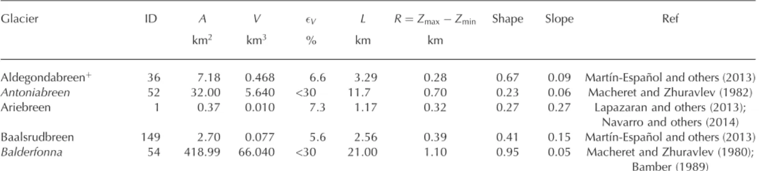
Table 7.Collection of glaciers used for constructing the scaling relationships presented in this paper. Glacier names in italics indicate that the volume has been taken from Cogley’s catalogue. A superscriptþnext to the glacier name indicates an updated volume estimate with respect to that given in Grinsted (2013), taken from Cogley’s catalogue. ID gives the glacier number as indicated in Figure 1.Ais area,Vis volume,V is the estimated error in volume,Lis the glacier length along its central flowline,R¼ZmaxZmin is the altitude range, and
‘Shape’ and ‘Slope’ are dimensionless quantities calculated asW=LandR=L, respectively, whereWis the average width of the glacier, given byA=L. ‘Ref’ is the data source. An asterisk next to an error in volume indicates that the error estimate has been taken from the original source. The area of Sveigbreen is smaller than that in the RGI because a branch of the glacier was not radio-echo sounded
Glacier ID A V V L R¼ZmaxZmin Shape Slope Ref
km2 km3 % km km
Aldegondabreenþ 36 7.18 0.468 6.6 3.29 0.28 0.67 0.09 Martín-Español and others (2013)
Antoniabreen 52 32.00 5.640 <30 11.7 0.70 0.23 0.06 Macheret and Zhuravlev (1982)
Ariebreen 1 0.37 0.010 7.3 1.17 0.32 0.27 0.27 Lapazaran and others (2013); Navarro and others (2014) Baalsrudbreen 149 2.70 0.077 5.6 2.56 0.39 0.41 0.15 Martín-Español and others (2013)
Balderfonna 54 418.99 66.040 <30 21.00 1.10 0.95 0.05 Macheret and Zhuravlev (1980);
Bamber (1989)