Simulation of the electrical operation of a lathe by using PI type regulators and
Bond-Graph technique.
Gregorio Romero, Jesus Felez, M. Luisa Martínez, Joaquín Maroto
ETSI Industriales, Univ. Politécnica de Madrid, José Gutiérrez Abascal, 2, 28006. Madrid, Spain
E-mail {gregorio.romero, jesus.felez, luisa.mtzmuneta, joaquin.maroto}@upm.es
Abstract - When designing circuits, engineers need to know the voltages and intensities at every point in the circuit. In simple circuits the results can be calculated by hand by using complex numbers, but in complex circuits this is impossible. This is why, nowadays, recourse is had to computer simulation so that circuits can be designed before being built, since it eliminates the need to build prototypes of the circuits with the ensuing time and cost.
Bond-Graph technique is a visual methodology that adds more transparency to the processes and it has turned out to be remarkably useful as it is a simple, effective method that can be applied to any physical system where there is a power exchange.
This work initially analyses the starting mechanism of a direct current machine using Bond Graph technique, compares it with a model developed in Simulink © and then stabilises the running of the motor by using a type PI controller.
Keywords – simulation; Bond Graph; electrical domain; lathe; DC motor; PI regulators.
I.INTRODUCTION
The use of such a machine as a generator or dynamo is practically obsolete since alternating current (AC) machines has more advantages for generating, transporting and distributing electrical energy than direct current (DC) machine due to the simplicity and low-cost of using transformers to convert one voltage to another. Another drawback to this machine is that it requires more maintenance than an asynchronous machine, since the friction of the brushes in the collector produces a great deal of wear.
Nevertheless, a DC machine has a greater degree of flexibility in controlling the speed and torque compared to AC machines. Such flexibility combined with its simplicity when analysing and simulating means it is highly suitable for applying to different industrial operating mechanisms, such as, for example, conventional lathes.
The Bond Graph technique enables systems belonging to the different areas of physics to be modelled in a way that is both intuitive and close to reality [1]. It is a perfect technique for representing elements belonging to the area dealt with in this paper. This paper presents an application by using Bond Graph technique to simulate the electrical operation of a lathe by using type PI regulators.
II.LATHE SIMULATION MODEL
The purpose of a lathe is to rotate a part that needs to be shaped. It comprises a DC electric motor that is joined to the part by means of a reduction gear which is subject to control.
The software used for simulating the Bond Graph
technique-based models is Bondin © [2]and, in order to
verify the results obtained, the same simulation is
performed in Simulink © [3], developing the block
diagrams of the equivalent system.
Figure 1. Equivalent circuit of a DC motor
The model to be developed requires an independently excited DC motor (fig. 1) and a shaft with a reduction gear. The initial work cycle will consist in the initial start-up of the machine until the nominal rotation of the part is reached, which is when the blade will act for a certain time by applying a load torque for a certain time followed by a deceleration of the motor at the same rhythm as during start-up. After stopping the lathe, the process is repeated but in the opposite direction.
A DC machine (generator or motor) basically comprises two parts; a stator, which provides the apparatus with mechanical support, and a space in the middle, usually cylindrical in shape.
From an electrical circuit point of view, DC machines comprise an inductor or excitation placed in the stator and a rotary armature fitted with a commutator segment collector placed at the rotor. On applying a DC excitation voltage
Uex to the inductor of the machine, an excitation current Iex
is produced, which, in turn, produces a flow Φ, which
causes an electromotive force E in the armature due to the movement of the rotor.
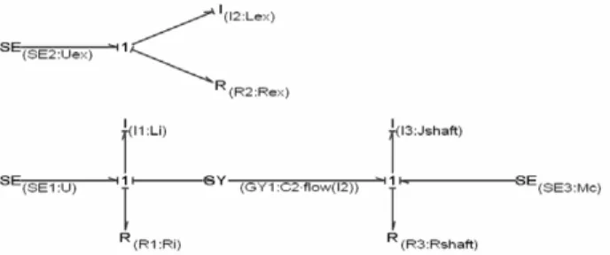
The representation of both windings in Bond-Graph technique [1] [5] is done by representing two circuits that are isolated but interdependent through magnetic flux. As figure 2 illustrates, the isolated part represents the inductor, which is dependent on the excitation voltage (Uex), in this case independently of the induced circuit, while the rest represents the armature of the motor and the rest of the lathe. As can be seen, the armature is dependent on the feed voltage (U) and on the flow in the inductor coil (flow (I2)), since the gyrator element is dependent on the exciter circuit. Ports R and L are the resistance and the inductance of the equivalent circuits of the motor.
Figure 2. Lathe model in a Bond Graph.
To obtain the full model, all that needs to be done is to
add the resistance torque Mc, which is an effort source
joined to the output shaft using a type 1 node since the flow or angular velocity is the same.
Having described the model to be simulated, the different operating parameters are as follows:
1000
380 2 075
14250 1000 1200
= = Ω = =
= = Ω =
= ⋅ = ⋅ = ⋅
i i 2
e e e
2 2
shaft shaft c
U V R 0,04 L 2 mH C 1 U V R , L 0,2 mH
J kg m R kg m M kN m
III.OPERATION OF A LATHE WITHOUT REDUCTION GEAR
We will firstly look at how it operates with the load connected directly to the drive shaft without any reduction gear in between.
In order to get the required start-up the input voltage
(U) and the load torque (Mc) should be formulated so that
they are variables in time. In this way, the DC motor start-up will occur during the first 2 seconds. During this interval the voltage is a ramp that reaches the nominal value at its end. It is at this instant that the nominal rotation speed is reached. In the period stretching from 2 to 10 seconds the voltage will remain constant. Finally, from 10 to12 seconds a ramp should be inserted into the voltage with the same gradient as during the start-up but with a negative sign, so that it will gradually decelerate until it stops.
Therefore, the voltage code is as follows:
if ((t>=0) and (t<2)) {U=500*t}; if ((t>=2) and (t<10)) {U=1000};
if ((t>=10) and (t<12)) {U=1000-500*(t-10)}; if (t>=12) {U=0};
The load torque generated by the friction of the blade against the rotating part should be inserted similarly so that it will be present when the nominal operating speed has been reached and outside the start-up and stopping periods, that is to say, during the 4 to 8 second interval:
if ((t>=0) and (t<4)) {Mc=0};
if ((t>=4) and (t<8)) {Mc=-1200000}; if (t>=8) {Mc=0};
Once the Bond Graph design model is known together with the voltage and load conditions over time, the simulation generates the following result:
Shaft rotation speed [rad/s]
Time [s]
Figure 3. Lathe speed during the work cycle
It it can be seen in figure 3 how the lathe reaches its nominal speed in the described time and how this is reduced as the load acts.
In order to validate the Bond-Graph model, the same
simulation was performed using Simulink ©. To do this, the
block diagram needs to be obtained from the system equations:
E dt di · L ·i R
U= i + i + (1)
dt dΩ · J M
-Mi c= eje (2)
By applying the Laplace transformation to the expressions (1) and (2) we get:
i i
U(s)=(R +L ·s)·I(s)+E(s) ↓
i
i i i
L
U(s)-E(s) (R L ·s)·I(s) 1 ·s ·R I(s)
i
R
⎛ ⎞
= + = +⎜ ⎟ ⋅
⎝ ⎠
↓
[
]
ii
1
U(s)-E(s) R I(s)
L
1 ·s
i
R
⋅ = ⋅
+ (3)
i c eje
Bearing in mind that in the expression (4) the torque is
proportional to the current (Mi= ⋅ ⋅k ΦIi), in the block
diagram both the torque on the shaft as well as the load torque should be represented as the corresponding intensity multiplied by Ri.
(
)
Φ ⋅ ⋅ ⋅ = − ⋅ Φ ⋅ k ) s ( E J s ) s ( I ) s ( Ik i c eje
↓
(
)
s E(s)k J R ) s ( I R ) s ( I
Ri i i c i eje2⋅ ⋅ Φ ⋅ ⋅ = ⋅ − ⋅ ↓
[
]
(
)
E(s)s J R k ) s ( I R ) s ( I R eje i 2 c i i
i ⋅ ⋅ =
Φ ⋅ ⋅ ⋅ − ⋅ (5)
The DC motor block diagram is then as follows:
Figure 4. DC motor block diagram
The gains ‘GainM’ and ‘GainO’ are constants that
transform the value ‘Ri·Ii’ into the corresponding torque
(Mi) and E into the angular velocity (Ω). They are
calculated using the following expressions:
i
R k GainM= ⋅Φ
(6) Φ ⋅ = k 1
GainO (7)
Once the preceding expressions have been examined, the system’s transfer functions are:
( )
·s T ·s 1R L · k· ·R J 1 U(s) E(s) m 2 i i 2 i
eje + +
Φ
= (8)
( )
( )
( )
·s 1k· ·R J ·s R L · k· ·R J ·s k· ·R J U(s) (s) ·R I 2 i eje 2 i i 2 i eje 2 i eje i i + Φ + Φ Φ
= (9)
( )
( )
k· ·s 1 ·R J ·s R L · k· ·R J 1 (s) ·R I (s) ·R I 2 i eje 2 i i 2 i eje i c i i + Φ + Φ= (10)
( )
( )
k· ·s 1 ·R J ·s R L · k· ·R J ·s) R L (1 (s) ·R I E(s) 2 i eje 2 i i 2 i eje i i i c + Φ + Φ + −= (11)
To substitute the values of the system under study, all
that needs to be known is ‘k·Φ’. In a steady state,
nom nom i nom
E =U -R ·I =1000-1044·0,04=958,24 V (12)
nom
nom nom
nom
E 958,24
E k·Φ· k·Φ 183,01 V·s
2π
Ω 50·
60
= Ω → = = = (13)
The value of ‘Ic·Ri’ should be calculated from the load
torque Mc:
i c i c
R 0,04
I R M 1200000× 262,28 V
k 183,01
⋅ = ⋅ = =
⋅Φ
(14)
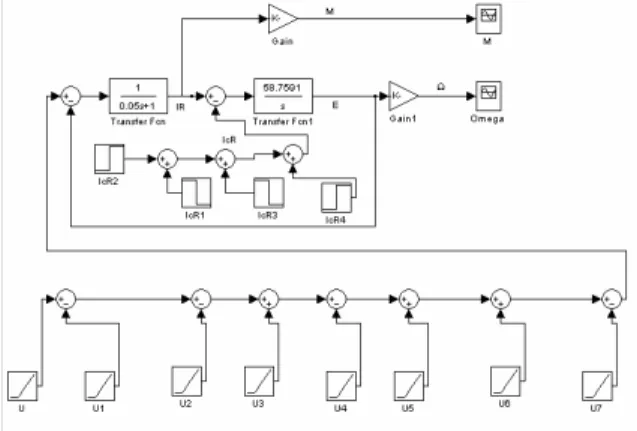
The input values U and ‘Ic·Ri’ should be entered into
Simulink © using a ramp sequence and the block diagrams will then be as in the following figure.
Figure 5. Lathe block diagram.
As the graph below illustrates, the results given by
Simulink © have the same value and shape as those obtained from the developed Bond-Graph model (figure 3).
Shaft rotation speed [rad/s]
Time [s]
In both cases (figures 3 and 6) rotation speed has been represented over time. We can see the acceleration period, rotation at constant speed, the drop in speed as a result of applying the load torque, speed recovery when the load torque is removed and the deceleration of the motor until it stops.
IV.OPERATION OF A LATHE WITH REDUCTION GEAR
In respect of the connection between the part and the motor described previously, this is usually done using a one stage reduction gear, there being two wheels with their respective moments of inertia ‘J’ and friction coefficients ‘R’, where ‘r’ is the transformation ratio between both. If a reduction gear is placed between the motor and the load, the Bond Graph model is slightly modified to what is shown in the following figure.
Figure 7. Lathe model with reduction gear in a Bond-Graph.
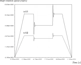
After inserting a r=1/1 and r=1/2 reduction, bearing in mind that the moments of inertia of each wheel are 500
kg·m2 and 2000 kg·m2 respectively, and that the friction of
both wheels is zero, the results given are those in the following figure.
Shaft rotation speed [rad/s]
Time [s]
Figure 8. Lathe speed with r=1/1 and r=1/2.
With the reduction gear, the nominal speeds are multiplied by the ratio of the reduction gear, as shown in figure 8. It can also be seen that the resistance effect of the
blade is four times less ((1/½)2) when the second speed ratio
is worked with.
In Simulink © the block diagram should look the same
as in figure 6, but the load input torque ‘Ic·Ri’ will have to
be substituted for ‘r·Ic ·Ri’ and the shaft inertia Jeje for
‘r2·J2+Jeje+J1’.
V.REGULATING THE DC MOTOR USING A PSEUDO BOND GRAPH-BASED PI.
In the two simulations performed it can be seen how the rotation speed drops as a result of applying load torque. For this reason, the main objective should be to control the system with a type PI regulator so that when the blade is applied to the part, the part recovers its operating speed.
PI
R1
R2
Ue
C1
R3
R4
Us
Figure 9. Electrical layout of the PI regulator.
This type of regulator is usually simulated [5] by building the model corresponding to the electrical circuit in figure 9, but contrary to what might be expected, when the
error tolerance is very small (10-5), and a simulation is
performed with the ‘Dassl’ algorithm [6] no satisfactory results are obtained because the solutions differ. For this reason, it was decided to build a Bond Graph model that would precisely and directly reproduce the PI functionality and not as had been attempted up to now by simulating its component parts.
In order to make an optimal model, Bondin © allows
working directly with the flow integral as the differential equation of the load in the coils and the voltage are directly generated.
As the pseudo Bond-Graph [1] [2] [4] in figure 10 shows, the voltage reaching the DC motor is regulated so that it is a function (Kp) proportional to the difference between the feed voltage (U) and the reference value and proportional to the integral of this reference (Ki). Therefore, when the load is applied to the shaft the rotation speed of the shaft will move away from the nominal value and the input voltage to the motor will be automatically controlled by the PI regulator shown.
Figure 10. Pseudo Bond Graph-based PI regulator model.
r=1/1
The pseudo Bond Graph-based model has been built so that the feed voltage value can be used as reference since it is compared with the product of the shaft rotation speed of the machine and the factor that makes it proportional to the
feed voltage under the nominal speed (183.15/r). This
model uses flow sources (SF1 and SFref) instead of effort
sources, which is logical, as in this way the integral and the variable associated with the Inertance port (I_in) that will then exist, can be easily obtained so that the corresponding proportional (Kp) and integral (Ki) constants can be applied.
In this way, the regulation of the DC motor by using the PI controller explained in these lines should be connected at the beginning of the reduction gear lathe model developed in the Bond-Graph in figure 7.
Figure 11. Bond Graph model of the motor with a PI regulator
When the regulator was set after having made various trials, it was found that for a value of Kp=300 and Ki=10, a regulation was automatically obtained, as can be seen in figures 12, 13 and 14.
Shaft rotational speed [rad/s]
Time [s]
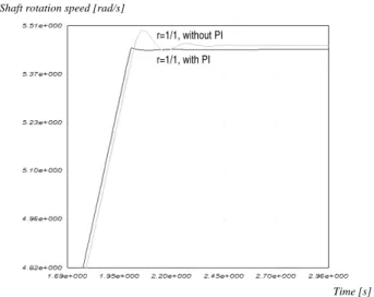
Figure 12. Lathe speed with r=1/1 and r=1/2 with/without PI.
If no controller is used, when the operating speed is reached the inertia of the machine causes it to over-accelerate a little and it takes 0.4 seconds to stabilise.
However, thanks to the regulator it can be seen (fig. 13) how it runs much more smoothly since the slight over-acceleration existing on attaining nominal speed has been eliminated and it now takes only 0.2 seconds to stabilise.
Shaft rotation speed [rad/s]
Time [s]
Figure 13. Detail of figure 12 with/without PI.
Figure14 shows in detail how the regulation system responds when the blade is applied by increasing the voltage input to the motor to compensate the negative torque being applied and so obtain nominal speed. Not only does the fluctuation of the rotation speed drop but also the stabilisation time.
Shaft rotation speed [rad/s]
Time [s]
Figure 14. Detail of figure 12 with/without PI.
As it can be seen when the regulator work it does the lathe runs much more smoothly, the fluctuations of the rotation speed drop and reduce the stabilisation time with different coefficients reduction.
r=1/1, with PI
r=1/1, without PI
r=1/2, with PI
r=1/2, without PI
r=1/1, without PI
r=1/1, with PI
r=1/1, with PI
VI.CONCLUSIONS.
Computer simulation leads to an understanding of how systems work without actually needing to see them. It may be said that the Bond Graph technique is a simple and effective mathematical modelling technique that lets the model be understood without losing the physical sense of each of its components, no matter how complex it may be. Its methodology unified for different physical domains enables the electrical part to be joined to other parts of the systems that appear in engineering, such as, mechanics or hydraulics, it being unnecessary to change the simulation environment or computer application when machines need to be joined to mechanical shafts, pumps or turbines,…
The advantage of the model developed here is that anyone who is simulating anything in Bond Graph software and wishes to adopt a model like the one shown here to connect it to the rest of the model does not need simulate it in any other tool; all that is needed is to transform the equation system to a Bond Graph or Pseudo Bond Graph model by using the different topology of the nodes and ports.
REFERENCES
[1] D.C. Karnopp, D.L. Margolis and R.C. Rosenberg. System Dynamics: a Unified Approach. 2nd Edition, Wiley Interscience, New York, 1990.
[2] G. Romero, J. Félez, J. Maroto and M.L. Martínez. “Simulation of an Asynchronous Machine by using a Pseudo Bond Graph“. AIP Conference Proceedings. Vol. 1060, Issue 1, pags 137-146. 2008.
[3] J.H. Mathews, F. Kurtis and K. Fink, Numerical Methods Using MatLab. Prentice Hall. 2004.
[4] José J. Granda and Nathaniel Kong. “Pseudo bond graph models and finite element models of transient heat transfer problems”. Intemational Conference on Bond Graph Modeling ICBGM'93. JJ.Granda and F.E.Cellier, eds San Diego, SCS Publishing, Simulation Series, Vol.25, No.2, pp.293-300. 1993.
[5] S. Junco, D. Marelli and M. Romero. “Bond Graph Modelling and Simulation of Electrical Machines”. Proceedings Int´l. Conf. MSO'97 (Singapore, Aug. 11-13), IASTED/Acta Press, Calgary, Canada 1997.