Leave and let leave: A sufficient condition to explain the
evolutionary emergence of cooperation
Luis R. Izquierdoa, Segismundo S. Izquierdob, Fernando Vega-Redondoc aDepartment of Civil Engineering, Universidad de Burgos, 09001 Burgos, Spain;
bDepartment of Industrial Organization, Universidad de Valladolid, 47011 Valladolid, Spain;
cDepartment of Decision Sciences and IGIER, Bocconi University, Via Roentgen 1, 20136 Milan, Italy;
PREPRINT
Formatted version at http://dx.doi.org/10.1016/j.jedc.2014.06.007
Abstract
The option to leave your current partner in response to his behavior, also known as
conditional dissociation, is a mechanism that has been shown to promote the emergence and stability of cooperation in many social interactions. This mechanism, nevertheless, has always been studied in combination with other factors that are known to support cooperation by themselves. In this paper, we isolate the effect of conditional dissociation on the evolution of cooperation and show that this mechanism is enough to sustain a significant level of cooperation if the expected lifetime of individuals is sufficiently long.
Graphical abstract:
Keywords: Option to leave; Conditional Dissociation; Prisoner’s dilemma; Positive assortment; Exit option.
JEL code: C73
Supplementary material: http://luis.izqui.org/models/LeLeLe/index.html
Corresponding Author: Luis R. Izquierdo
Universidad de Burgos, Edificio la Milanera, C/ Villadiego s/n,09001, Burgos, Spain Tel: +34 947 259410; Fax: +34 947 258910
1.
Introduction
The issue of how cooperation can evolve in social dilemmas has long been a central research topic in modern evolutionary theory.1 Many alternative routes have been proposed to explain such a “paradox,” often modeling the question in terms of individuals involved in an iterated Prisoner’s Dilemma. In this context, some of the mechanisms considered have been, for example, schemes for punishing defectors, local or preferential interactions among selected members (e.g. kin selection, tag-based groups or spatial structure), tit-for-tat-like reciprocity, or selective matching based on memory or reputation.
Most of these alternatives presume what, in some biological contexts, may be considered as rather advanced cognitive capacities.2 In social contexts, on the other hand, the fact that sophisticated behavior in humans should be conceived as costly naturally raises the question of whether cooperation can emerge and be sustained also through very simple mechanisms.3
One particularly stark answer to this question is provided in this paper. Specifically, we show that the option to leave a partner in response to his action can just by itself provide an evolutionary basis for the rise of cooperation. It does so by generating endogenous positive assortment –i.e., a high probability of interacting with someone who plays the same action as you do (Bergstrom, 2003; Rivas, 2013)–, even if the matching mechanism is completely random, under conditions that we will characterize precisely.
More specifically, our model studies a dynamic population of cooperators and defectors who repeatedly interact to play a Prisoner’s Dilemma, and remain together in couples until one of them decides to leave or dies. There is, therefore, the potential for voluntary (conditional) dissociation: after each round of play, individuals may decide to leave their partner or stay with him, depending on the latter’s action. This delineates a scenario with only eight different possible strategies, in which we simply postulate that their respective frequencies vary according to relative success (i.e. the average payoffs they earn). In this context, our main conclusion can be succinctly stated as follows: it is sufficient that the expected lifetime of individuals be long enough for a significant extent of cooperation to emerge and stabilize in the long run –either globally (from any initial conditions) if the expected lifetime is sufficiently long, or only locally (around the unique cooperative equilibrium) for intermediate lifetime values.
A key role in our results is played by the strategy that always cooperates and breaks the relationship immediately if, and only if, the partner defects. We shall label this behavior as
cooperative conditional dissociation, where the term “dissociation” (in contrast to “association”) emphasizes that individuals use their capacity to discard their current partner but have no control over the new one. 4 Essentially this same strategy –or closely related
1 See Nowak (2006) and Bowles and Gintis (2011) for recent surveys of this literature from complementary
perspectives.
2 For example, Bergmüller et al. (2010) provide many biological examples where cooperation has evolved in
species where individual animals display little or no behavioral plasticity.
3 There is a relatively large literature that, following the lead of Rubinstein (1986) and Abreu and Rubinstein
(1988), studies the implications of complexity costs in the behavior displayed by agents playing the repeated Prisoner’s Dilemma. In fact, a significant fraction of this literature has pursued an evolutionary approach. Binmore and Samuelson (1992), Cooper (1996), Volij (2002) and van Veelen & García (2010) are some representative examples, differing in a number of important modeling details. They also differ in their respective conclusions, which range from the possibility of supporting full cooperation to the impossibility of supporting any at all. None of these papers, however, contemplates a scenario where voluntary dissociation is an option and the matching pool is adjusted accordingly.
4 This was also the term we used in a preceding paper (Izquierdo et al., 2010), which studied this behavior in a
substantially more complex scenario. In particular, besides the option to leave a partnership, agents could also change their behavior within a given (maintained) relationship in response to their partner’s preceding behavior.
variants– has been studied before in the literature under different names. Noteworthy examples are CONCO (Schuessler, 1989), Out-for-Tat (Hayashi, 1993), MOTH (Joyce et al., 2006) or Walk Away (Aktipis, 2004).5
The customary approach of this literature has been to show, through computationally implemented contests, that such a strategy can prevail and hence promote cooperation when confronted with different specific subsets of other strategies –for example, suitably adapted versions of Tit-for-Tat or the so-called Pavlov. Albeit insightful in many respects, this methodology is not best suited to attain a clear-cut analysis of the effects and mechanics of conditional dissociation in the promotion of cooperation. Since this is the primary purpose of this paper, we propose instead a “minimalist setup” that, while including the option to leave or stay in response to partner’s behavior, remains instead devoid of any other considerations that could cloud the key forces at work. In such a setup, we ask the following two basic questions: Can conditional dissociation alone give rise to cooperative behavior? If so, what are the dynamic (evolutionary) properties of the mechanism induced by conditional dissociation? To answer these questions, we purposely focus on the simplest strategy space that allows for conditional dissociation in an unbiased manner and nothing else, i.e. one where individuals are either cooperators or defectors, and they can only condition their decision to leave on their partner’s behavior. This admittedly simplistic setting seems the natural starting point to assess whether the appearance of a certain trait –i.e. conditional dissociation– may provide an initial footing for the evolutionary emergence of cooperation, since evolution tends to gradually move from simplicity to greater sophistication, rather than the other way around. Nonetheless, the question of whether the potential appearance of greater behavioral complexity –in the form of more sophisticated strategies– may destabilize cooperation will also be addressed at the end of the paper (see Section 6 and Appendix A).
We end this introduction by relating our model to that studied by Fujiwara-Greve and Okuno-Fujiwara (2009) –hereafter referred to as FO– which is the closest to our approach. In line with the work by Ghosh and Ray (1996), Kranton (1996), or Carmichael and Macleod (1997), FO consider an infinitely large population of agents who play the repeated Prisoner’s Dilemma and always have the option of voluntary separation and re-match. They conduct a thorough static analysis of this voluntarily separable repeated Prisoner’s Dilemma without restrictions on the strategy space, other than assuming that individuals do not know the past history of their new partners when re-matching, i.e., players can react to any possible history of actions taken in their current partnership.6
FO’s approach and ours are complementary. On the one hand, our strategy space is much simpler than theirs but, on the other hand, this purposefully self-imposed restriction allows us to analyze the dynamics of the model. To be clear, FO investigate evolutionary stability following a static approach, which leads to a characterization of equilibria under certain
That paper, therefore, combines conditional dissociation with other strategic considerations and hence does not provide a sharp understanding of that mechanism. See below a similar point concerning related literature. 5 Further interesting examples where conditional dissociation or an exit option has been shown to promote cooperation in networks are Pacheco et al. (2006), Santos et al. (2006) and, in experimental studies, Boone and Macy (1999), Coricelli et al. (2004), or Hauk and Nagel (2001). Also related is the study of continuous-action social dilemmas where there is a co-evolution of a player’s level of contribution to the partnership and the minimum contribution she requires from her partner in order not to break the partnership (McNamara et al., 2008; Sherratt and Roberts, 1998).
6 In a recent independent paper, Fujiwara-Greve and Okuno-Fujiwara (2012) consider whether cooperation can
be supported by immediate voluntary separation alone. Even allowing for other more general strategies, they find that such support of cooperation is possible (in a neutrally stable configuration), provided entrants are restricted to being trust-building equilibrium entrants in the sense of Swinkels (1992). We elaborate further on this question in section 6 of this paper, where we discuss different issues of robustness.
idealized conditions (including, among others, the assumption of infinite populations and a strict separation between the timescales at which selection and mutation operate). While the static analysis provides very useful insights, its results cannot be directly applied to any real system –for which, by definition, some of the idealized hypotheses do not apply. Perhaps more importantly, the static analysis is silent about the tendency of the evolutionary process to gravitate towards one equilibrium or another, about the effect of initial conditions on the dynamic path followed by the system and on its end points (Huttegger and Zollman, 2013), about the possible transitions that may occur among different equilibria over time, or about the effect that mutation may have on the displacement or even the existence of dynamic attractors. These are some of the aspects that we address in our analysis.
The rest of the paper is organized as follows. First, in Section 2, we provide a detailed description of the evolutionary process on a given finite population. Next, in Section 3, we conduct some exploratory computer simulations that anticipate and illustrate our main conclusion, namely, that the system is able to support a high-cooperation regime if, and only if, individuals’ expected lifetime is long enough. The following two sections summarize the main theoretical analysis of the model. In Section 4 we carry out a static analysis that follows the approach undertaken in FO. As explained, this static analysis provides candidate centers of attraction for the dynamics of the process under some limiting conditions. In particular, we identify (a) the set of Nash equilibria of an underlying population game and (b) the subset of Nash equilibria that are neutrally stable.
Section 5 contains the core of our analysis. In it we conduct a dynamic analysis of the system and show that its behavior is well captured by the mean dynamics (Sandholm, 2010), particularly in terms of convergence to one of two possible attractors (a defective one and a partially cooperative one). The location and characteristics of these attractors are determined for different mutation rates. We find that a comparative analysis on the effect of the parameters of the model is fully in line with intuition, i.e. both the basin of attraction of the cooperative attractor and the extent of cooperation it displays grow with the expected lifetime of individuals. In Section 6 we discuss the robustness of our results to changes in two notorious simplifying assumptions of our model, namely the limited size of the strategy space and the absence of matching friction.
The paper ends in Section 7 with the conclusions. For the sake of smooth exposition, the detailed proofs of our results are relegated to Appendix A, while in Appendix B we study a variation of the model that includes matching friction. This latter appendix confirms that none of our conclusions are affected if the re-matching mechanism allows for either some delay and/or some outside payoff.
2.
The model
We consider an evolutionary model of conditional dissociation where a finite population of individuals interact in pairs in every period to play a Prisoner’s Dilemma. Their strategies have three components. The first component X1 ∈ {C, D} determines whether the individual
is a cooperator or a defector in all of his interactions. The second component X2 ∈ {L, S}
specifies whether he leaves or stays with his current partner after the latter has cooperated, while the third component X3 ∈ {L, S} specifies an analogous choice after the current partner
has defected. Overall, such a range of behavior gives rise to a strategy set 𝚲 consisting of eight possible strategies for each individual, X1X2X3 ∈{C, D} × {L, S}2.
We formulate the model in discrete time. Within each period, the following sequence of events takes place in order:
1. The individuals who enter the period being single are randomly matched in pairs to form new partnerships, while the rest continue to interact with their previous partners.
2. The pair of individuals involved in each partnership play a Prisoner’s Dilemma. Each of them chooses his action (C or D) as determined by the first component of their respective strategy. They then obtain their corresponding payoff, as follows: if both cooperate, they receive R (Reward); if both defect, P (Punishment); if one cooperates and the other defects, the cooperator obtains S (Sucker) and the defector obtains T (Temptation). As usual, the aforementioned payoffs are assumed to satisfy T>R>P>S≥ 0.
3. Each individual independently decides whether to stay in his current partnership or leave (S or L), as prescribed by the two last components of his strategy –i.e., by the second component if the partner has cooperated, or by the third component if the partner has defected. If an individual chooses to leave, his current partnership is broken and both players involved in it move to the pool of singles.
4. Every individual dies with probability (1-δ) –a stochastically independent event across individuals. Hence δ is the one-step survival rate, which leads to an individual’s expected lifetime given by f = (1-δ)-1. If only one individual in a partnership dies, his partner enters the pool of singles.
5. Dead individuals are immediately replaced by new entrants. (Thus, for simplicity, the size of the population remains constant, but this assumption is inessential.) The entrants independently copy the decision rules of the individuals who played the game in the current period; the probability that any particular individual’s strategy will be copied is proportional to the individual’s payoff in the current period –“reproductive fitness,” therefore, is proportional to payoffs. There is, however, a small probability µ of “mutation” for every entrant, in which case his strategy becomes equal to any particular strategy 𝑠 ∈ 𝚲 with probability ms > 0. Naturally, entrants are temporarily placed in the pool of singles.
The process described above defines a stochastic Markov process in which the state of the system can be chosen to be the number of partnerships that display each possible strategy pair {𝑠,𝑠′} after the matching has taken place (i.e. right after stage 1 above). Our analysis will focus on studying the fraction of strategies of each type that prevail in the long run. As advanced, a prominent role will be played by the strategy CSL that prescribes cooperative behavior and has the individual stay with his partner if and only if the latter also cooperates. This strategy embodies the intuitive idea of “cooperative conditional dissociation”.7
3.
Some illustrative simulations
In this section we illustrate the essential features of the model through some representative parameterizations. The model requires specifying the following set of parameters: the population size N, the payoffs in the game, the one-step survival probability 𝛿 (or, equivalently, the expected lifetime f), the probability of mutation 𝜇 ∈[0,1], and the probabilities ms of mutating to each strategy s. As a typical case for medium or large populations, we show results for N = 400, [T = 4, R = 3, P = 1, S = 0], 𝜇 = 0.05 and ms = 1/8. Let xCC be the fraction of CC outcomes, or “level of cooperation,” and let us define xDD and
xCD similarly. Simulations of this process for short expected lifetimes (f < 8) present a quick evolution towards a situation where the level of cooperation is almost null (xCC ≈ 0, while xDD
7 Note that models confronting strategies where dissociation is not allowed (i.e. CSS vs. DSS), or where
dissociation is not conditional (i.e., including CLL and DLL), cannot lead to any degree of cooperation.
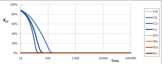
is close to 1) –i.e., a non-cooperative regime is reached, as displayed in Fig. 1. The reader can replicate all simulation results presented in this paper by using the applet provided in the supplementary material.
Fig. 1. Evolution of the fraction of CC outcomes for 8 different runs with short expected lifetime (f = 5), each run starting with the whole population using one of the 8 different strategies. Parameterization: N = 400, T = 4, R = 3, P = 1, S = 0, µ = 0.05, ms = 1/8.
In stark contrast, for long expected lifetimes (f > 30), and after some periods of adjustment, the simulations evolve towards a situation with a significant level of cooperation –i.e. a cooperative regime–, as displayed in Fig. 2. We show below that the level of cooperation xCC
in this cooperative regime can be well approximated by a reference value xCC*
that is
calculated from the mean dynamics equations provided in Section 5. The most prevalent strategies at this polymorphic regime are CSL and DSL, followed by DLL.
Fig. 2. Evolution of the fraction of CC outcomes for 8 different runs with long expected lifetime (f = 50), each run starting with the whole population using one of the 8 different strategies. Parameterization: N = 400, T = 4, R = 3, P = 1, S = 0, µ = 0.05, ms = 1/8.
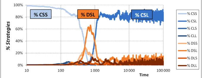
To gain intuition on the dynamic competition among strategies taking place in the simulation runs summarized in Fig. 2, consider Fig. 3, which shows the evolution of each strategy share in one representative run starting with the whole population using strategy CSS.
Fig. 3. Evolution of the fraction of individuals using each strategy in one representative run with long expected lifetime (f = 50), starting with the whole population using strategy CSS. Parameterization: N = 400, T = 4, R = 3, P = 1, S = 0, µ = 0.05, ms = 1/8.
The initial population of naïve CSS cooperators is soon invaded by defective strategies – notably DSL– who are able to exploit CSS without mercy. However, such exploitation cannot last long, since naïve cooperators obtain very low payoffs and, consequently, evolutionary pressures select against them. As CSS individuals die off, DSL exploiters find it harder to thrive, and CSL individuals are then able to take over by avoiding long exploitations (when matched with defective strategies) and establishing stable cooperative partnerships mostly with each other.
For intermediate values of the expected lifetime f, the process typically evolves towards either the cooperative or the non-cooperative regime, with possible transitions between them (Fig. 4). In general, starting from random conditions, there is an initial tendency of the process to approach the non-cooperative regime, but then –especially for high values of f – a transition to a longer-lasting cooperative regime often occurs.
Fig. 4. Evolution of the fraction of CC outcomes for 8 different runs with intermediate expected lifetime (f = 20), each run starting with the whole population using one of the 8 different strategies. Parameterization: N = 400, T = 4, R = 3, P = 1, S = 0, µ = 0.05, ms = 1/8.
The time series shown above provide useful insights on the dynamics of the model, but a proper understanding of the problem requires a systematic analysis of the model under the whole range of possible parameter values. This is what we do in the next two sections. To this end, we follow a common approach in the literature and consider limit scenarios for the following three key variables: population size N, mutation rate 𝜇, and time t. 8
Concerning the population size, the analysis focuses on the case where N is very large –that is, formally, we maintain the assumption that it can be well approximated by a continuum. Then, concerning the other two variables, 𝜇 and t, we conduct two different limit exercises. First, in Section 4, we focus our analysis on the stationary states that may prevail in the asymptotic time limit, under the implicit assumption that the mutation rate 𝜇 is positive but infinitesimally small. Formally, this amounts to considering those stationary configurations of the mutation-free dynamics that are evolutionarily robust to some infrequent mutation (see below for a formal definition). As already explained, this exercise is inherently static. Therefore, in Section 5 we turn our attention to the study of the evolutionary dynamics in full interplay with the mutation process. This is done through the study of a set of mean dynamics equations where the processes of selection and mutation operate on the same time scale (with the latter working at a rate that can be small but is always positive).
4.
Static analysis
Our static analysis of the model is based on the concepts and results developed by FO, suitably adapted to our context. This involves, in particular, the restriction to our strategy space 𝚲, which rules out the possibility that individuals may display any action plasticity when playing the Prisoner’s Dilemma with a given partner. Specifically, this implies that in the matching stage the stationary strategy distributions in the pool of singles are of the form
𝒙 ∈ 𝒫(𝚲), where 𝒫(𝚲) denotes the set of all strategy distributions in our model (which coincides with the 7-simplex; thus we may make 𝒫(𝚲) ≡ Δ7).
Given any such distribution 𝒙 assumed to be stationary, one can define the average payoff
𝜋�𝑠(𝒙) obtained by any given strategy 𝑠 ∈ 𝚲. On the basis of these payoffs, FO define the concepts of Nash Distribution (ND) and Neutrally Stable Distribution (NSD), whose counterpart in our case can be defined as follows:
Definition 1. Nash Distribution (ND) A stationary strategy distribution in the matching pool
𝒙 ∈ 𝒫(𝚲) is a Nash Distribution if for all 𝑠 ∈ 𝑠𝑢𝑝𝑝(𝒙) and 𝑠′∈ 𝚲,
𝜋�𝑠(𝒙)≥ 𝜋�𝑠′(𝒙)
Definition 2. Neutrally Stable Distribution (NSD) A stationary strategy distribution in the matching pool 𝒙 ∈ 𝒫(𝚲) is a Neutrally Stable Distribution if, for any 𝑠′ ∈ 𝚲, there exists
𝜀̅ ∈(0,1) such that for any 𝑠 ∈ 𝑠𝑢𝑝𝑝(𝒙) and any 𝜀 ∈(0,𝜀̅),
𝜋�𝑠�(1− 𝜀)𝒙+𝜀𝒔′� ≥ 𝜋�𝑠′�(1− 𝜀)𝒙+𝜀𝒔′�
where 𝒔′∈ 𝒫(𝚲) is the strategy distribution consisting only of strategy 𝑠′.
8 It is well understood that, in evolutionary models, the order in which these limits are taken often leads to
fundamentally different conclusions (see Beggs, 2002; Binmore and Samuelson, 1997; Binmore et al., 1995; Sandholm, 2010). Thus, in general, the particular order being chosen must depend on the specific question being posed and the right theoretical framework to address it.
Using these concepts, we prove the following results for our model (see Appendix A):
Proposition 1. Assume 𝛿 > 0 and let
𝛿𝑀𝑖𝑛 =�(𝑅 − 𝑆)(𝑃 − 𝑆𝑇 − 𝑆) +�(𝑇 − 𝑅)(𝑇 − 𝑃)< 1
𝜓= 𝑃+𝑅 −2𝑃𝛿2 + (𝑆+𝑇)(−1 +𝛿2)
Then, the set of all Nash distributions can be characterized as follows:
a) If 𝛿 <𝛿𝑀𝑖𝑛, it consists of all strategy distributions whose support contains defective
strategies only.
b) If 𝛿 ≥ 𝛿𝑀𝑖𝑛, it includes both the set of strategy distributions specified in (a), as well as
the set of partially cooperative distributions where a fraction 𝛼 ∈ (0,1) of the players choose CSL and the other (1− 𝛼) fraction of the players choose DSL and/or DLL, with the following two possible values for 𝛼:
𝛼 =2(𝑇 − 𝑃1 )𝛿2(𝜓 ± �𝜓2−4(𝑇 − 𝑃)𝛿2(𝑃 − 𝑆)(1− 𝛿2))
Proposition 2. Let 𝛿𝑀𝑖𝑛 be defined as in Proposition 1. Among the Nash Distributions
identified there, the subset of Neutrally Stable Distributions can be characterized as follows.
a) If 𝛿 ≤ 𝛿𝑀𝑖𝑛, it consists of all strategy distributions whose support contains defective
strategies only.
b) If 𝛿 >𝛿𝑀𝑖𝑛, it includes both the set of strategy distributions specified in (a), as well as
the set of partially cooperative distributions where a fraction 𝛼 ∈ (0,1) of the players choose CSL and the other (1− 𝛼) fraction of the players choose DSL and/or DLL, where 𝛼 is given by:
𝛼 =2(𝑇 − 𝑃1 )𝛿2(𝜓+ �𝜓2−4(𝑇 − 𝑃)𝛿2(𝑃 − 𝑆)(1− 𝛿2))
The level of cooperation xCC given by the fraction of cooperating pairs is xCC = 0 in case (a), whilst at the partially cooperative NSDs it is given by:
𝑥cc= 𝛼 2
1− 𝛿2(1− 𝛼2).
The present (static) evolutionary analysis of the system singles out two sets of NSDs –a non-cooperative equilibrium set and a partially non-cooperative one– and characterizes the level of cooperation in each of them. As we will show in the next section, these two sets of equilibria constitute the centers of attraction for the dynamics of our system if the mutation rate is small (under the maintained assumption that the population is very large). This will represent the first step in our dynamic analysis. Building on it, our objective will be to shed light on the following two important respects:
i) The behavior of the system over time. Specifically, we shall provide the closed-form equations that approximate the dynamics of the system from its initial conditions to its long-run behavior in a continuous fashion.
ii) The impact of mutation on the existence, location, and strategy composition of the centers of attraction. In general, it is clear that, if mutation is not truly negligible, some of the NSDs may constitute a poor approximation of the regimes actually displayed by our system. To illustrate this possibility, consider for instance the simulations depicted in Fig. 2, which were conducted for a mutation rate 𝜇 = 0.05. There we find that for large values of the expected lifetime, the non-cooperative NSD becomes a very poor predictor of the long-run behavior of the process, even if the system departs from it and remains for many periods with a very low level of cooperation. As a different illustration, refer to the simulations shown in Fig. 4, corresponding to the same mutation rate. There we see that the partially cooperative regime induces an average level of cooperation xCC = 68%, which contrasts with the predicted level if one uses the cooperative NSD (xCC = 86%) for the same expected lifetime.
In the following section we present an analytical approximation to the dynamics of the system that will help address the previous questions. In particular, it will identify the centers of attraction and accurately describe the expected behavior of the system over time for any given mutation rate 𝜇. We will also show that the limiting rest points of the approximated dynamics (as 𝜇 →0) must correspond to Nash distributions, hence providing a link between the static equilibria and the evolutionary dynamics.
5.
Mean dynamics
As explained before, we may regard the evolutionary process described in Section 2 as a Markov chain whose states specify the number of partnerships associated to each possible strategy pair right after the matching stage. Given the population size, an equivalent way of representing a state of this process is in terms of the vector 𝒑 = [𝑝𝑠,𝑠′] that specifies, for every possible pair of strategies 𝑠,𝑠′ ∈ 𝚲, the fraction𝑝𝑠,𝑠′ of individuals in the whole population who are choosing strategy 𝑠 and are paired with an individual who is choosing strategy 𝑠′. Naturally, 𝑝𝑠,𝑠′= 𝑝𝑠′,𝑠 and ∑ 𝑝𝑠,𝑠′ 𝑠,𝑠′ = 1, so 𝒑contains 35 independent variables.
This is indeed a complicated system to describe and analyze exhaustively. To tackle the problem, we shall follow the customary approach of focusing the analysis on its expected motion. This gives rise to the so-called mean dynamics, which is expected to be a good approximation of the stochastic evolution of the original Markov chain when the population is large and the process changes gradually (Sandholm, 2010).
In essence, the mean dynamics approach is based on the presumption that, since the original (finite-state) Markov process embodies a collection of stochastically independent events in every period, its mean (deterministic) counterpart can suitably approximate aggregate behavior if the population is large. In practice, such a deterministic law of motion is built upon an identification of the following pairs of ex ante and ex post magnitudes:
a) ex ante matching probabilities and ex post frequencies at the pairing stage,
b) expected number of deaths and average number of deaths for each group of strategists, c) ex ante mutation probabilities and ex post frequencies.
As explained below, such identification allows the formulation of the mean dynamics which, at each point in time, reflects the expected motion of the original process.
As a first step, we start by calculating the expected law of motion for each frequency 𝑝𝑠,𝑠′. To do this, we shall find it useful to denote by 𝚽 the set of strategy pairs that induce a stable partnership:
𝚽= � 〈𝐶𝑆𝑆〈𝐶𝐿𝑆,,𝐷𝑆𝑆〉𝐶𝑆𝑆〉,,〈𝐶𝐿𝑆〈𝐶𝑆𝑆,,𝐷𝑆𝐿〉𝐶𝑆𝐿〉,,〈𝐶𝑆𝑆〈𝐷𝑆𝑆,,𝐷𝑆𝑆〉𝐷𝑆𝑆〉,,〈𝐶𝑆𝑆〈𝐷𝑆𝑆,,𝐷𝑆𝐿〉𝐷𝐿𝑆〉,,〈𝐶𝑆𝐿〈𝐷𝐿𝑆,,𝐶𝑆𝐿〉𝐷𝐿𝑆〉�,
and then introduce the corresponding indicator function: we need information on the payoffs earned by the different strategies. Let 𝜋(𝑠,𝑠′) stand for the stage payoff obtained by strategy 𝑠 ∈ 𝚲 in a partnership with strategy 𝑠′∈ 𝚲, and denote by 𝜋�𝑠(𝒑) =𝑝1𝑠∑𝑠′∈𝚲𝑝𝑠,𝑠′𝜋(𝑠,𝑠′) the average payoff obtained by players choosing 𝑠 ∈ 𝚲 under 𝒑 –here, for expositional simplicity, we assume that 𝑝𝑠 = ∑𝑠′∈𝚲𝑝𝑠,𝑠′> 0 for all 𝑠 ∈ 𝚲. Further denote by 𝜋�(𝒑) =∑𝑠∈𝚲𝑝𝑠·𝜋�𝑠(𝒑) the average payoff earned by individuals across the whole population. Then, within the mean dynamics framework, the fractions 𝑦𝑠(𝑡) can be computed as follows (dispensing with the explicit dependence on t from the right-hand side):
𝑦𝑠(𝑡) = (1− 𝛿)�(1− 𝜇)𝑝𝑠𝜋�𝜋�(𝑠𝒑()𝒑)+𝜇𝑚𝑠�+𝛿2∑ �𝑖∈Λ 1− ϕ𝑠,𝑖�𝑝𝑠,𝑖+𝛿(1− 𝛿)𝑝𝑠 [2] where each of the terms in the right-hand side of [2] corresponds in turn to:
1. newborn 𝑠-strategists;
2. surviving 𝑠-strategists involved in broken partnerships where the partner also survived; 3. surviving 𝑠-strategists whose partner died (regardless of whether the partnership was stable
or not).
A combination of [1] and [2] also allows us to find an expression for the expected motion of the population frequency of each strategy 𝑠 (again, dependence on t is omitted on the right-hand side):
Accounting now for the fact that the period length is taken to become infinitesimally small, that defines a continuous-time mean dynamics that approximates the original discrete-time stochastic evolutionary process described in Section 2. Such a dynamical system on the frequencies of strategy pairs can easily be seen to lead to an aggregate dynamics on the marginal frequencies of individual strategies given by
𝑑𝑝𝑠(𝑡)
𝑑𝑡 = (1− 𝛿)�(1− 𝜇)
𝑝𝑠(𝑡)𝜋�𝑠(𝒑)
𝜋�(𝒑) +𝜇𝑚𝑠− 𝑝𝑠(𝑡)� . [4]
As a preliminary step in our dynamic analysis, it is interesting to compare the stationary points of [4] with the game-theoretic equilibrium notions considered in the previous section.9
Naturally, to carry out this comparison in a meaningful manner, we must consider a context where the mutation rate µ is small (albeit positive), i.e., we focus on configurations that are labeled limit stationary states. Mathematically, these are identified with the limit of a sequence of stationary states obtained as 𝜇 → 0 (see Samuelson, 1997), and constitute a strict subset of the stationary states for 𝜇= 0. (As an example, the cooperative monomorphic distributions are stationary states of the mean dynamics with 𝜇 = 0, but they are not limit stationary states.) We obtain the following result:
Proposition 3. Assume 𝑚𝑠 > 0 ∀𝑠 ∈ 𝚲. A limit stationary state 𝒑∗ of the mean dynamics
induces a stationary strategy distribution in the matching pool, 𝒙∗ ∈ ∆𝟕, that is a Nash
Distribution.
This result implies that, in striving to identify the long-run predictions of the dynamic process for low mutation rates in large populations, it is enough to restrict attention to those stationary states that induce Nash Distributions in the matching pool of singles. Intuitively, it can be seen as the dynamic counterpart of the result stated in Proposition 2 for the static analysis –i.e. in both cases, we find that Nash behavior is a necessary condition for evolutionary stability. Now, however, rather than refining Nash equilibrium through a static evolutionary concept such as NSD, we shall rely on a genuinely dynamic approach to the problem. Specifically, we shall turn our attention to the time paths induced by the mean dynamics on the marginal distribution of strategy frequencies, as captured by [4].
In Figures 5-7 below we present the time paths [𝑝𝑠]𝑠∈Λ for the same parameter values under which we conducted the simulations respectively described by Figures 1, 2 and 4 in Section 3. We observe that the mean dynamics provide an effective way of smoothly tracing the behavior displayed by the simulations under the different parameter configurations considered. This illustrates that, as advanced, the (deterministic) mean approach represents a useful tool to study the (stochastic) behavior generated by the original evolutionary process when the population is large. For a more exhaustive comparison, these two dynamics –the mean dynamics and the stochastic evolutionary process– can be compared side by side using the applet provided in the supplementary material for any parameter value.
9 Note that, in contrast with the static approach, here stationarity is not assumed, but derived as a property that
only a small subset of states display for the explicit dynamics given by equation [4].
Fig. 5. Time paths for the fraction of CC outcomes in the mean dynamics equations, for 8 different initial conditions with short expected lifetime (f = 5); each path starts with the whole population using one of the 8 different strategies. Parameterization: T = 4, R = 3, P = 1, S = 0, µ = 0.05, ms = 1/8.
Fig. 6. Time paths for the fraction of CC outcomes in the mean dynamics equations, for 8 different initial conditions with long expected lifetime (f = 50); each path starts with the whole population using one of the 8 different strategies. Parameterization: T = 4, R = 3, P = 1, S = 0, µ = 0.05, ms = 1/8.
Fig. 7. Time paths of the fraction of CC outcomes in the mean dynamics equations, for 8 different initial conditions with intermediate expected lifetime (f = 20); each path starts with the whole population using one of the 8 different strategies. Parameterization: T = 4, R = 3, P = 1, S = 0, µ = 0.05, ms = 1/8.
We now summarize a systematic numerical exploration of the limit behavior induced by the mean dynamics equations. We considered different parameterizations [T, R, P, S, µ > 0, ms > 0] and, for each of them, explored a wide range of different values of the expected lifetime f
starting from a fine grid of initial conditions 𝒑(𝑡= 0). This analysis revealed the existence of two threshold values for the expected lifetime, f1 and f2, (dependent on the specific parameterization) such that: 10
i) If f < f1, all the trajectories converge to a stationary state characterized by a vanishing fraction of CC outcomes (i.e. a value of xCC close to 0) – see Fig. 5. We label such a situation the non-cooperative attractor.
ii)If f1 ≤ f < f2, the trajectories converge either to a non-cooperative stationary state as before, or to an alternative one characterized by a high fraction of CC outcomes, which we label as the cooperative attractor –see Fig. 7 for an illustration. Denote by xCC*(f) the fraction of cooperating pairs in this attractor, which is a function of the expected life f. The higher the value of f, the higher the value of xCC* (f), as well as the larger it is the basin of attraction of the corresponding cooperative attractor (i.e. the set of initial conditions from which the dynamical system converges to the cooperative attractor). iii) If f ≥ f2, all trajectories converge to a cooperative attractor, whose fraction of cooperating
pairs again displays a monotonically increasing relationship with the expected lifetime f – see Fig. 6.
Given that the mean dynamics equations constitute a good (continuous and deterministic) approximation of the original evolutionary process, we can use them to uncover interesting properties of the original stochastic model. As a particularly interesting example, consider the clear-cut mean-dynamics prediction that, when the expected lifetime f renders cooperation possible, the system is eventually absorbed by one of two attractors: a non-cooperative attractor where the level of cooperation essentially vanishes, and a cooperative attractor displaying a well-defined level of cooperation that is uniquely associated to the underlying parameters. Does the discrete evolutionary process admit a similarly dichotomous categorization of the possible long-run outcomes? In what follows, we confirm that this is indeed the case.
A first conceptual problem in addressing the issue is how to define the counterparts of the cooperative and non-cooperative attractors in the discrete evolutionary process where, by its stochastic nature, even any aggregate predictions must be subject to some residual noise. To this end, we formally define two regimes: a Cooperative Regime (CR) and a Non-Cooperative Regime (NCR), each defined in terms of the corresponding attractors as follows. First, for the CR, we identify a state in the discrete process to be part of this regime if its level of cooperation (measured by the fraction xCC of cooperating pairs) is close to the level xCC*(f) displayed asymptotically by the mean dynamics for the same value of f and the other underlying parameters. More specifically, we require that |xCC - xCC*(f)| < 0.1, where a band width amounting to 20% of the population is simply chosen for concreteness. A similar approach is undertaken in order to define the NCR for the discrete process, a state being defined to lie in the NCR if its fraction xDD of non-cooperating pairs satisfies xDD > 0.8.
Fig. 8 shows that, even for a moderate population size (N = 400) with regular inflow of mutants (µ = 0.05), the categorization of the two regimes in terms of their mean-dynamics counterparts is remarkably successful in condensing the actual dynamics of the process for
10 Focusing, for concreteness, on the representative parameterization of payoffs given by [T = 4, R = 3, P = 1, S =
0], and setting ms = 1/8, we provide here the values of f1 and f2, for different mutation rates: {µ = 0.05, f1 = 9, f2
= 38}; {µ = 0.01, f1 = 8, f2 = 182};{µ = 0.001, f1 = 8, f2 > 1000}.
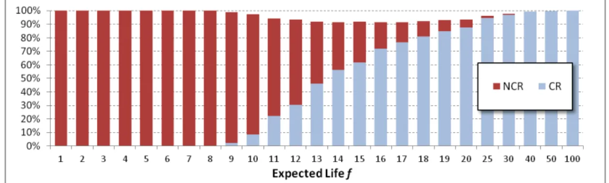
every value of the expected lifetime f. The two regimes always span more than 90% of the time of the process, and therefore represent a good dichotomous description of its evolution. As expected from our mean-dynamics analysis, when the parameter configuration is such that the two regimes coexist, their relative importance depends on the expected life. Specifically, we find that the NCR completely dominates the long-run behavior of the process for low values of f (i.e. f < f1µ=0.05= 9) and then the CR gradually gains time share until the level of f
= f2µ=0.05 = 38, critical value from which the CR essentially becomes fully dominant. Heuristically, this can be seen as the reflection of the impact that f has on relative strength (depth and size) of the “basins of attraction” of the cooperative and non-cooperative regimes (i.e. on the probability that a randomly selected initial condition leads to either of them).
Fig. 8. Fraction of periods spent in the Cooperative (CR) and Non-Cooperative (NCR) Regimes as a function of the expected lifetime f. The values in each column are compiled over 103 simulation runs. Every run is measured
between periods 3·103 and 104, with random initial conditions. N = 400, T = 4, R = 3, P = 1, S = 0, µ = 0.05, m s =
1/8.
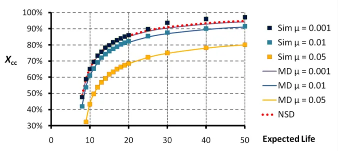
A complementary perspective on the issue is provided by Fig. 9, where we compare the level of cooperation in the CR obtained in simulations of the original process (Sim) and the corresponding level of cooperation induced by the mean dynamics (MD). (For completeness, we also include the prediction of the static analysis that is embodied by the NSD concept.) It is remarkable that, despite the fact that the band that is used to define the CR for the discrete evolutionary process is quite narrow (i.e. xCC*(f) ± 0.1), the induced average level of
cooperation is very well captured by the mean-dynamics prediction, even with mutation rates that span an order of magnitude. This observation can be regarded as further evidence that, despite the unavoidable noise, the behavior displayed by the discrete process is well anchored around the corresponding mean-dynamics predictions.
Fig. 9. Level of cooperation in the cooperative regime of the stochastic simulations (Sim) and in the cooperative attractor of the mean dynamics (MD) for different values of the expected life and mutation rate µ. The isolated points (Sim) correspond to average values computed from simulations of the original stochastic process as in Fig. 8. For comparison, we also include the predicted level of cooperation in the cooperative Neutrally Stable Distribution (NSD). Parameterization: N = 400, T = 4, R = 3, P = 1, S = 0, ms = 1/8.
Another issue of interest is to understand what strategies support each of the two regimes, both in the medium and in the long run. In the medium run, some strategies can play a key role as a temporary bridge to attain the regime in question from given initial conditions. Instead, in the long run, other strategies can be the ones needed to sustain the regime in a stationary manner (recall the dynamics shown in Fig. 3). Again, the mean dynamics can be used to shed light on this issue and hence clarify the results obtained in actual implementations of the original stochastic process. For the Cooperative Regime CR, we find that a typical path of the mean dynamics is as shown in Fig. 10. Initially, in a heterogeneous population, defection gains population share through sophisticated defectors (i.e. those who, by playing the strategy DSL, exploit naïve cooperators by staying with them, but immediately quit other defectors.) But this adaptation eventually saturates and self-imposes a bound on how much it can profit from such a behavior. At this point, sophisticated cooperators (who stay with cooperators but abandon defectors) take over and dominate in the long run, at the induced steady state.
Fig. 10. Time paths of the fraction of individuals using each strategy in one run of the mean dynamics equations starting from initial conditions where the 8 strategies are equally represented, and converging to the cooperative attractor. Parameterization: f = 20, T = 4, R = 3, P = 1, S = 0, µ = 0.01, ms = 1/8.
Concerning such long-run cooperative behavior, it is interesting to see how the strategy profile at the cooperative attractor depends on the parameters of the model –most importantly, on the expected lifetime. Fig. 11 shows the distribution of strategies in the cooperative attractor of the MD when µ = 0.01, under different values of the expected lifetime f. The analogous figure for the discrete evolutionary process is basically identical, so we do not include it here. We see that there is a clear predominance of CSL, followed by DSL and DLL. Thus, as illustrated also in Fig. 10, the simple and intuitive strategy that stays with a cooperator but abandons a defector is the key cornerstone on which cooperation is sustained in the CR across all relevant values of the expected lifetime f. In contrast, for the non-cooperative regime, all the defective strategies can be found, with a predominance of DSL in general. When defection is the dominant behavior, no significant differences in behavior follow from alternative defection-based strategies.
Fig. 11. Composition of strategies in the cooperative attractor. Parameterization: T = 4, R = 3, P = 1, S = 0, µ = 0.01, ms = 1/8.
6.
Robustness
In this section, we discuss the robustness of our results to changes in two prominent simplifying features of our model, i.e. the assumption of immediate re-matching and the limited size of our strategy space. While we clarify that introducing re-matching frictions would not affect the gist of our analysis, the limits imposed on the strategy space are explained to be essential. In fact, we argue that some such limits are unavoidable if one wants to find a compromise between non-existence and wide-range multiplicity. In this sense, our sharp limitation to strategies that focus on dissociation alone appears a natural choice to achieve the aim of our analysis.
Let us consider first the specification of the matching mechanism operating in every period. Our simplifying assumption in this respect has been that the players who enter the pool of singles are immediately re-matched, i.e. there are no delay frictions in finding a partner. In general, it may be natural to posit that not all players in the pool of singles are re-matched with probability one every period and that, when single players remain unmatched, they receive only a relatively low payoff. Would this variation reduce the level of cooperation? In Appendix B we show that this is not the case; intuitively, note that defectors tend to suffer a greater number of separations, and thus incur in higher re-matching costs. Hence the model happens to be robust to the consideration of those matching frictions.
Turning now to extensions on the strategy space, let us discuss the static stability of distributions in the unrestricted strategy space. First of all, it should be noted that the partially cooperative regime composed by strategies CSL, DSL and DLL is not robust to entrants of any complexity; to be precise, it does not constitute a NSD in the unrestricted strategy space. Consider, for instance, the so-called 1-period trust-building strategy C1, which starts defecting, keeps the partnership if and only if its partner also defects in their first interaction, and from then onwards stays and cooperates indefinitely if and only if its partner also cooperates –otherwise it leaves (Fujiwara-Greve and Okuno-Fujiwara, 2009). Following the arguments put forward by FO (2009, pg. 1005), it can be shown that the deviation made by C1
is profitable when compared with DSL and DLL, i.e. C1 can always invade the (1− 𝛼) share of DSL-DLL (Fujiwara-Greve and Okuno-Fujiwara, 2012).11 Elaborating upon this idea, we
next show that any reasonably strong result on stability within this framework will require some constraints on the strategy space.
In the unrestricted space of strategy distributions with finite support, we prove in Appendix A.6 that if the expected life is sufficiently long, no strategy distribution can be Robust Against Indirect Invasions (RAII; van Veelen, 2012), consequently precluding any other stronger stability concept such as evolutionary stability.12,13 In other words, there is always a chain of
neutral mutants that can open the door to an invasion. Consequently, the situation in the unrestricted framework with an option to leave is analogous to that pointed out by van Veelen & García (2010) for the standard iterated prisoner’s dilemma: if the discount factor or continuation probability is large enough, every equilibrium can be upset, either by a mutant –
11 Clearly, if other restrictions on the strategy space are considered, this equilibrium can regain certain stability.
For instance, Fujiwara-Greve and Okuno-Fujiwara (2012) show that the equilibrium formed by CSL and DLL constitutes an evolutionarily stable distribution under trust-building equilibrium entrants, in the sense of Swinkels (1992).
12 The set of strategy distributions with finite support is the set of distributions in which the number of pure
strategies that can be played is finite. In particular, this set includes all strategies distributions made up of a finite number of mixed strategies with finite support.
13 Robustness against indirect invasion is a stability criterion that is weaker than evolutionary stability and
stronger than neutral stability (van Veelen, 2012).
if the equilibrium is not neutrally stable–, or by a succession of mutants –if it is neutrally stable.
Focusing on the weaker stability concept of NSDs, the nonexistence situation is reversed in the sense that there are an infinite number of such distributions. In particular, FO identify a family of NSDs made up of the so-called trust-building strategies, though many of these equilibria have been shown not to be robust to within-partnership mixed strategy entrants (Vesely & Yang, 2012).14
7.
Conclusion
Our model shows that, in contexts where agents have some control over the continuation of their partnerships, even the simplest form of conditional dissociation can induce cooperation in the Prisoner’s Dilemma through the operation of the standard evolutionary forces (selection and mutation). The “disciplinary mechanism” that constrains the spread of defection in this context is simply the possibility of terminating a relationship with a defecting party. And this abandonment acts as enough punishment because, when the system is in a Cooperative Regime (CR), the proportion of defectors in the pool of singles is much greater than the proportion of defectors in the population.
All the cooperative strategies present at significant levels in the CR are non-exploitable in the sense that they immediately leave a defecting partner. Defectors, therefore, are almost constantly changing partner, while pairs of cooperators usually remain together for much longer, thus generating some positive assortment. Heuristically, the role of this phenomenon is to introduce some endogenous adverse-selection, analogous to the classical Gresham’s law (Rolnick and Weber, 1986) –i.e., worn-out, torn, or generally low-quality notes are found mainly in circulation, whilst notes that are in better shape are preferentially kept in wallets and safes. Similarly, in the CR the pool of singles concentrates a higher than average proportion of defectors (i.e. low-quality individuals), often “in circulation”, while cooperators (i.e. high-quality partners) are mainly found playing in stable couples within a largely separate segment of the “market.”
When strategies of any complexity are allowed, it turns out that there is no finite distribution that is robust against indirect invasions. In other words, given any finite distribution, one can always find a sequence of neutral mutant distributions (or mixed strategies) that can open the door to a full invasion.
8.
Acknowledgements
We would like to thank Prof. Ken Binmore for many helpful comments and discussions. We are also very grateful to an anonymous reviewer for constructive comments and suggestions. We acknowledge financial support from projects ACCESS (EU, 12-120610), SIMULPAST (MICINN, CSD2010-00034) and SPPORT (JCyL, VA056A12-2). L.R.I. is very grateful to the Spanish Ministry of Education for grant JC2009-00263. A large part of this work was developed at the Economics Department of the European University Institute. L.R.I. and S.S.I. are very grateful for their kind hospitality.
14 A strategy distribution in the pool of singles is equivalent to a mixed strategy which randomly selects one of
the pure strategies in its support at the beginning of every new partnership. We use the term “within-partnership mixed strategy” to refer to those strategies which, at every period within a partnership, can choose with some probability –conditional on the outcome history within the partnership– whether to play C or D, and, likewise, whether to leave or stay.
Appendix A. Proofs
Appendix A is organized as follows: A.1. Notation and definitions
A.2. Lemma 1
A.3. Proof of Proposition 1 A.4. Proof of Proposition 2
A.4.a. Strategy distributions whose support contains defective strategies only
A.4.b. Partially cooperative ND 𝑥𝛼,𝛽 where a fraction 𝛼 ∈(0,1) of the players are CSLs A.4.c. The level of cooperation at the partially cooperative NSDs
A.5. Proof of Proposition 3
A.6. Nonexistence of RAII distributions A.6.a. Introduction
A.6.b. Definition (Evolutionarily equal and better performers). A.6.c. Definition (RAII distributions).
A.6.d. Proposition 4.
A.1. Notation and definitions
Strategies. Let 𝚲 be the set of possible strategies, 𝚲𝐂≡ {𝐶𝑆𝑆,𝐶𝑆𝐿,𝐶𝐿𝑆,𝐶𝐿𝐿} the set of cooperative strategies, and 𝚲𝐃 ≡ {𝐷𝑆𝑆,𝐷𝑆𝐿,𝐷𝐿𝑆,𝐷𝐿𝐿} the set of defective strategies. Let 𝚽 denote the set of stable strategy pairs, and ϕ𝑠,𝑠′ the corresponding indicator function, as defined in Section 5. Let 𝒫(𝚲) be the set of all strategy distributions in the population.
Expected Partnership Length. Let 𝐿(𝑠,𝑠′) be the expected length of the partnership of
𝑠 ∈ 𝚲 and 𝑠′ ∈ 𝚲, measured in number of periods. Note that 𝐿(𝑠,𝑠′) =�1−ϕ𝑠,𝑠′𝛿2�−1.
Average payoff at stationary distributions. Let 𝑥𝑖 denote the share of individuals with strategy 𝑖 ∈ 𝚲 in the matching pool. Let 𝒙 = {𝑥𝑖}𝑖∈Λ ∈ 𝒫(𝚲) be a stationary strategy distribution in the matching pool. Then, the average payoff 𝜋�𝑠(𝒙) obtained by strategy s in a stationary strategy distribution 𝒙 is (Fujiwara-Greve and Okuno-Fujiwara, 2009):
𝜋�𝑠(𝒙) =∑𝑖∈𝚲∑ 𝑥𝑥𝑖 ·𝐿(𝑠,𝑖) ·𝜋(𝑠,𝑖) 𝑖 ·𝐿(𝑠,𝑖) 𝑖∈𝚲
where 𝜋(𝑠,𝑖) is the per-period payoff obtained by strategy s in a partnership with strategy 𝑖.
A.2. Lemma 1
Lemma 1 formalizes the intuitive notion that it is best to stay with cooperators and leave defectors.
Lemma 1. Let 𝒙 ∈ 𝒫(𝚲) be a stationary strategy distribution in the matching pool. Then, for every 𝑠𝐶 ∈ 𝚲𝐂 and every 𝑠𝐷 ∈ 𝚲𝐃:
𝜋�𝐶𝑆𝐿(𝒙)≥ 𝜋�𝑠𝐶(𝒙); 𝜋�𝐷𝑆𝐿(𝒙)≥ 𝜋�𝑠𝐷(𝒙)
Furthermore, if 𝒙 ∈int(𝒫(𝚲)), then for every 𝑠𝐶 ≠ 𝐶𝑆𝐿 and every 𝑠𝐷 ≠ 𝐷𝑆𝐿:
𝜋�𝐶𝑆𝐿(𝒙) >𝜋�𝑠𝐶(𝒙); 𝜋�𝐷𝑆𝐿(𝒙) >𝜋�𝑠𝐷(𝒙).
Proof of Lemma 1
Note that for strategy distribution in the matching pool 𝒙 ∈ ∆7,every 𝑠
𝐶 ∈ 𝚲𝐂 and every
𝑠𝐷 ∈ 𝚲𝐃:
𝜋�𝑠𝐶(𝒙) =𝑅
∑𝑖∈𝚲𝐂𝑥𝑖·𝐿(𝑠𝐶,𝑖)
∑𝑖∈𝚲𝑥𝑖 ·𝐿(𝑠𝐶,𝑖) +𝑆
∑𝑖∈𝚲𝐃𝑥𝑖 ·𝐿(𝑠𝐶,𝑖)
∑𝑖∈𝚲𝑥𝑖 ·𝐿(𝑠𝐶,𝑖)
𝜋�𝑠𝐷(𝒙) =𝑇
∑𝑖∈𝚲𝐂𝑥𝑖 ·𝐿(𝑠𝐷,𝑖)
∑𝑖∈𝚲𝑥𝑖 ·𝐿(𝑠𝐷,𝑖) +𝑃
∑𝑖∈𝚲𝐃𝑥𝑖 ·𝐿(𝑠𝐷,𝑖)
∑ 𝑥𝑖∈𝚲 𝑖 ·𝐿(𝑠𝐷,𝑖) Let 𝑥𝐶(𝑠;𝒙) and 𝑥𝐷(𝑠;𝒙) be defined as follows:
𝑥𝐶(𝑠;𝒙) =∑∑𝑖∈𝚲𝐂𝑥𝑥𝑖·𝐿(𝑠,𝑖)
𝑖·𝐿(𝑠,𝑖)
𝑖∈𝚲 𝑥𝐷(𝑠;𝒙) =
∑𝑖∈𝚲𝐃𝑥𝑖·𝐿(𝑠,𝑖)
∑𝑖∈𝚲𝑥𝑖·𝐿(𝑠,𝑖) = 1− 𝑥𝐶(𝑠;𝒙)
𝑥𝐶(𝑠;𝒙) can be interpreted as the expected fraction of one-shot game interactions where the partner of an 𝑠-strategist will cooperate, and 𝑥𝐷(𝑠;𝒙) can be interpreted as the expected fraction of one-shot game interactions where the partner will defect.
Note that for every 𝑠𝐶,𝑠𝐶′ ∈ 𝚲𝑪 and every 𝑠𝐷,𝑠𝐷′ ∈ 𝚲𝑫:
𝐿(𝐶𝑆𝐿,𝑠𝐶′)≥ 𝐿(𝑠𝐶,𝑠𝐶′); 𝐿(𝐶𝑆𝐿,𝑠𝐷′) ≤ 𝐿(𝑠𝐶,𝑠𝐷′);
𝐿(𝐷𝑆𝐿,𝑠𝐶′) ≥ 𝐿(𝑠𝐷,𝑠𝐶′); 𝐿(𝐷𝑆𝐿,𝑠𝐷′)≤ 𝐿(𝑠𝐷,𝑠𝐷′);
Also, for every 𝑠𝐶 ∈ 𝚲𝑪,𝑠𝐶 ≠ 𝐶𝑆𝐿, there exists a strategy 𝑠(𝐶𝑆𝐿,𝑠𝐶) ∈ 𝚲such that: { 𝑠(𝐶𝑆𝐿,𝑠𝐶)∈ 𝚲𝑪 AND 𝐿(𝐶𝑆𝐿,𝑠(𝐶𝑆𝐿,𝑠𝐶)) > 𝐿(𝑠𝐶,𝑠(𝐶𝑆𝐿,𝑠𝐶)) } OR
{ 𝑠(𝐶𝑆𝐿,𝑠𝐶)∈ 𝚲𝑫 AND 𝐿(𝐶𝑆𝐿,𝑠(𝐶𝑆𝐿,𝑠𝐶)) < 𝐿(𝑠𝐶,𝑠(𝐶𝑆𝐿,𝑠𝐶)) }
Informally, the inequalities above state that, when comparing CSL with any other cooperative strategy 𝑠𝐶, CSL either stays strictly longer than 𝑠𝐶 with some cooperative strategy, or stays strictly less than 𝑠𝐶 with some defective strategy (or both).
Similarly, for every 𝑠𝐷 ∈ 𝚲𝑫,𝑠𝐷 ≠ 𝐷𝑆𝐿, there exists a strategy 𝑠(𝐷𝑆𝐿,𝑠𝐷)∈ 𝚲such that: { 𝑠(𝐷𝑆𝐿,𝑠𝐷) ∈ 𝚲𝑪 AND 𝐿(𝐷𝑆𝐿,𝑠(𝐷𝑆𝐿,𝑠𝐷)) > 𝐿(𝑠𝐷,𝑠(𝐷𝑆𝐿,𝑠𝐷)) }
OR
{ 𝑠(𝐷𝑆𝐿,𝑠𝐷) ∈ 𝚲𝑫 AND 𝐿(𝐷𝑆𝐿,𝑠(𝐷𝑆𝐿,𝑠𝐷)) < 𝐿(𝑠𝐷,𝑠(𝐷𝑆𝐿,𝑠𝐷)) }
The set of inequalities indicated above are sufficient to prove that for every 𝑠𝐶 ∈ 𝚲𝑪:
� 𝑥𝑖𝐿(𝐶𝑆𝐿,𝑖)
𝜋�𝐶𝐿𝑆(𝒙𝑵𝑫) =𝑅((𝑥𝑥𝐶𝑆𝑆+𝑥𝐶𝑆𝐿+𝑥𝐶𝐿𝑆+𝑥𝐶𝐿𝐿) +𝑆(𝛾𝑥𝐷𝑆𝑆 +𝛾𝑥𝐷𝑆𝐿+𝑥𝐷𝐿𝑆+𝑥𝐷𝐿𝐿) 𝐶𝑆𝑆+𝑥𝐶𝑆𝐿+𝑥𝐶𝐿𝑆+𝑥𝐶𝐿𝐿) + (𝛾𝑥𝐷𝑆𝑆 +𝛾𝑥𝐷𝑆𝐿+𝑥𝐷𝐿𝑆+𝑥𝐷𝐿𝐿)
≤ 𝑅((𝑥𝑥𝐶𝑆𝑆+𝑥𝐶𝑆𝐿+𝑥𝐶𝐿𝑆+𝑥𝐶𝐿𝐿) +𝑆(𝑥𝐷𝑆𝑆+𝑥𝐷𝑆𝐿+𝑥𝐷𝐿𝑆+𝑥𝐷𝐿𝐿)
𝐶𝑆𝑆+𝑥𝐶𝑆𝐿+𝑥𝐶𝐿𝑆+𝑥𝐶𝐿𝐿) + (𝑥𝐷𝑆𝑆 +𝑥𝐷𝑆𝐿 +𝑥𝐷𝐿𝑆+𝑥𝐷𝐿𝐿) = 𝜋�𝐶𝐿𝐿(𝒙𝑵𝑫)
< 𝑇((𝑥𝑥𝐶𝑆𝑆+𝑥𝐶𝑆𝐿+𝑥𝐶𝐿𝑆+𝑥𝐶𝐿𝐿) +𝑃(𝑥𝐷𝑆𝑆+𝑥𝐷𝑆𝐿+𝑥𝐷𝐿𝑆+𝑥𝐷𝐿𝐿) 𝐶𝑆𝑆+𝑥𝐶𝑆𝐿+𝑥𝐶𝐿𝑆+𝑥𝐶𝐿𝐿) + (𝑥𝐷𝑆𝑆+𝑥𝐷𝑆𝐿+𝑥𝐷𝐿𝑆+𝑥𝐷𝐿𝐿) = 𝜋�𝐷𝐿𝐿(𝒙𝑵𝑫)
ND.2. 𝐷𝑆𝑆 ∉ 𝑠𝑢𝑝𝑝(𝒙𝑵𝑫), since that would mean that 𝑥
𝐷𝑆𝑆 > 0 and, bearing in mind that
�∃𝑠𝐶 ∈ 𝚲𝑪 | 𝑥𝑠𝐶 > 0�, it would be the case that 𝜋�𝐷𝑆𝑆(𝒙𝑵𝑫) <𝜋�𝐷𝑆𝐿(𝒙𝑵𝑫). The proof follows
(assuming 𝑥𝐷𝑆𝑆 > 0 and �∃𝑠𝐶∈ 𝚲𝑪 | 𝑥𝑠𝐶 > 0�):
𝜋�𝐷𝑆𝑆(𝒙𝑵𝑫) =𝑇((𝛾𝑥𝛾𝑥𝐶𝑆𝑆+𝑥𝐶𝑆𝐿+𝛾𝑥𝐶𝐿𝑆+𝑥𝐶𝐿𝐿) +𝑃(𝛾𝑥𝐷𝑆𝑆+𝑥𝐷𝑆𝐿+𝛾𝑥𝐷𝐿𝑆+𝑥𝐷𝐿𝐿) 𝐶𝑆𝑆+𝑥𝐶𝑆𝐿+𝛾𝑥𝐶𝐿𝑆+𝑥𝐶𝐿𝐿) + (𝛾𝑥𝐷𝑆𝑆+𝑥𝐷𝑆𝐿 +𝛾𝑥𝐷𝐿𝑆+𝑥𝐷𝐿𝐿) <𝑇((𝛾𝑥𝛾𝑥𝐶𝑆𝑆+𝑥𝐶𝑆𝐿+𝛾𝑥𝐶𝐿𝑆+𝑥𝐶𝐿𝐿) +𝑃(𝑥𝐷𝑆𝑆 +𝑥𝐷𝑆𝐿 +𝑥𝐷𝐿𝑆+𝑥𝐷𝐿𝐿)
𝐶𝑆𝑆+𝑥𝐶𝑆𝐿+𝛾𝑥𝐶𝐿𝑆+𝑥𝐶𝐿𝐿) + (𝑥𝐷𝑆𝑆+𝑥𝐷𝑆𝐿+𝑥𝐷𝐿𝑆+𝑥𝐷𝐿𝐿) =𝜋�𝐷𝑆𝐿(𝒙𝑵𝑫)
ND.3. 𝐷𝐿𝑆 ∉ 𝑠𝑢𝑝𝑝(𝒙𝑵𝑫), since that would mean that 𝑥
𝐷𝐿𝑆 > 0 and, bearing in mind that
�∃𝑠𝐶 ∈ 𝚲𝑪 | 𝑥𝑠𝐶 > 0�, it would be the case that 𝜋�𝐷𝐿𝑆(𝒙𝑵𝑫) <𝜋�𝐷𝐿𝐿(𝒙𝑵𝑫). The proof follows
(assuming 𝑥𝐷𝐿𝑆 > 0 and �∃𝑠𝐶 ∈ 𝚲𝑪 | 𝑥𝑠𝐶 > 0�):
𝜋�𝐷𝐿𝑆(𝒙𝑵𝑫) =𝑇((𝑥𝑥𝐶𝑆𝑆+𝑥𝐶𝑆𝐿+𝑥𝐶𝐿𝑆+𝑥𝐶𝐿𝐿) +𝑃(𝛾𝑥𝐷𝑆𝑆+𝑥𝐷𝑆𝐿+𝛾𝑥𝐷𝐿𝑆+𝑥𝐷𝐿𝐿) 𝐶𝑆𝑆+𝑥𝐶𝑆𝐿+𝑥𝐶𝐿𝑆+𝑥𝐶𝐿𝐿) + (𝛾𝑥𝐷𝑆𝑆+𝑥𝐷𝑆𝐿+𝛾𝑥𝐷𝐿𝑆+𝑥𝐷𝐿𝐿) < 𝑇((𝑥𝑥𝐶𝑆𝑆+𝑥𝐶𝑆𝐿+𝑥𝐶𝐿𝑆+𝑥𝐶𝐿𝐿) +𝑃(𝑥𝐷𝑆𝑆+𝑥𝐷𝑆𝐿+𝑥𝐷𝐿𝑆+𝑥𝐷𝐿𝐿)
𝐶𝑆𝑆+𝑥𝐶𝑆𝐿+𝑥𝐶𝐿𝑆+𝑥𝐶𝐿𝐿) + (𝑥𝐷𝑆𝑆+𝑥𝐷𝑆𝐿+𝑥𝐷𝐿𝑆+𝑥𝐷𝐿𝐿) = 𝜋�𝐷𝐿𝐿(𝒙𝑵𝑫)
Thus, statements ND.1-3 above prove that the only strategies that could potentially be part of the support of 𝒙𝑵𝑫 are CSS, CSL, DSL, and DLL. Now consider the following facts:
ND.4. CSS and DSL cannot be both in the support of 𝒙𝑵𝑫 since that would mean that 𝑥 𝐶𝑆𝑆 > 0 and 𝑥𝐷𝑆𝐿 > 0, and then it would be the case that 𝜋�𝐶𝑆𝑆(𝒙𝑵𝑫) <𝜋�𝐶𝑆𝐿(𝒙𝑵𝑫). The proof follows (assuming 𝑥𝐶𝑆𝑆 > 0 and 𝑥𝐷𝑆𝐿 > 0):
𝜋�𝐶𝑆𝑆(𝒙𝑵𝑫) =𝑅((𝛾𝑥𝛾𝑥𝐶𝑆𝑆+𝛾𝑥𝐶𝑆𝐿+𝑥𝐶𝐿𝑆+𝑥𝐶𝐿𝐿) +𝑆(𝛾𝑥𝐷𝑆𝑆+𝛾𝑥𝐷𝑆𝐿+𝑥𝐷𝐿𝑆+𝑥𝐷𝐿𝐿) 𝐶𝑆𝑆+𝛾𝑥𝐶𝑆𝐿+𝑥𝐶𝐿𝑆+𝑥𝐶𝐿𝐿) + (𝛾𝑥𝐷𝑆𝑆+𝛾𝑥𝐷𝑆𝐿+𝑥𝐷𝐿𝑆+𝑥𝐷𝐿𝐿) < 𝑅((𝛾𝑥𝛾𝑥𝐶𝑆𝑆+𝛾𝑥𝐶𝑆𝐿+𝑥𝐶𝐿𝑆+𝑥𝐶𝐿𝐿) +𝑆(𝑥𝐷𝑆𝑆 +𝑥𝐷𝑆𝐿 +𝑥𝐷𝐿𝑆 +𝑥𝐷𝐿𝐿)
𝐶𝑆𝑆+𝛾𝑥𝐶𝑆𝐿+𝑥𝐶𝐿𝑆+𝑥𝐶𝐿𝐿) + (𝑥𝐷𝑆𝑆+𝑥𝐷𝑆𝐿+𝑥𝐷𝐿𝑆+𝑥𝐷𝐿𝐿) =𝜋�𝐶𝑆𝐿(𝒙𝑵𝑫)
ND.5. CSS and DLL cannot be both in the support of 𝒙𝑵𝑫 since that would mean that 𝑥 𝐶𝑆𝑆 > 0 and 𝑥𝐷𝐿𝐿 > 0, and then it would be the case that 𝜋�𝐷𝐿𝐿(𝒙𝑵𝑫) <𝜋�𝐷𝑆𝐿(𝒙𝑵𝑫). The proof follows (assuming 𝑥𝐶𝑆𝑆 > 0 and 𝑥𝐷𝐿𝐿 > 0):
𝜋�𝐷𝐿𝐿(𝒙𝑵𝑫) =𝑇((𝑥𝑥𝐶𝑆𝑆+𝑥𝐶𝑆𝐿+𝑥𝐶𝐿𝑆+𝑥𝐶𝐿𝐿) +𝑃(𝑥𝐷𝑆𝑆+𝑥𝐷𝑆𝐿+𝑥𝐷𝐿𝑆+𝑥𝐷𝐿𝐿) 𝐶𝑆𝑆+𝑥𝐶𝑆𝐿+𝑥𝐶𝐿𝑆+𝑥𝐶𝐿𝐿) + (𝑥𝐷𝑆𝑆+𝑥𝐷𝑆𝐿 +𝑥𝐷𝐿𝑆 +𝑥𝐷𝐿𝐿)
<𝑇((𝛾𝑥𝛾𝑥𝐶𝑆𝑆+𝑥𝐶𝑆𝐿+𝛾𝑥𝐶𝐿𝑆+𝑥𝐶𝐿𝐿) +𝑃(𝑥𝐷𝑆𝑆 +𝑥𝐷𝑆𝐿 +𝑥𝐷𝐿𝑆+𝑥𝐷𝐿𝐿) 𝐶𝑆𝑆+𝑥𝐶𝑆𝐿+𝛾𝑥𝐶𝐿𝑆+𝑥𝐶𝐿𝐿) + (𝑥𝐷𝑆𝑆+𝑥𝐷𝑆𝐿+𝑥𝐷𝐿𝑆+𝑥𝐷𝐿𝐿) =𝜋�𝐷𝑆𝐿(𝒙𝑵𝑫)
The five statements above (ND.1-5) together prove that the only strategies that could potentially be part of the support of a partially cooperative ND 𝒙𝑵𝑫 are CSL, DSL, and DLL. Thus, let us parameterize all possible (partially cooperative) mixtures of strategies {CSL,
DSL, DLL} using a generic distribution 𝒙𝜶,𝜷 where a fraction 𝛼 ∈(0,1) of the players are
CSLs and the other (1− 𝛼) of the players are DSLs and/or DLLs, in proportions determined by 𝛽 ∈[0,1] according to the following formula:
𝒙𝜶,𝜷= 𝛼𝒔𝑪𝑺𝑳+ (1− 𝛼)(𝛽𝒔𝑫𝑺𝑳+ (1− 𝛽)𝒔𝑫𝑳𝑳)
where 𝒔𝒊 is the strategy distribution consisting only of i-strategists. Note that DSL and DLL are behaviorally identical in 𝒙𝜶,𝜷 for any 𝛼 ∈(0,1) and 𝛽 ∈[0,1]. The payoffs for each strategy in 𝒙𝜶,𝜷 are (for any 𝛽 ∈[0,1]):
𝜋�𝐶𝑆𝐿�𝒙𝜶,𝜷�=
𝛼1−𝛿𝑅2+ (1− 𝛼)𝑆 𝛼1−𝛿1 2+ (1− 𝛼) · 1
𝜋�𝐷𝑆𝐿�𝒙𝜶,𝜷�= 𝜋�𝐷𝐿𝐿�𝒙𝜶,𝜷�=𝛼𝛼𝑇· 1 + (1+ (1− 𝛼− 𝛼)) · 1 =𝑃 𝛼𝑇+ (1− 𝛼)𝑃
A necessary condition to be a ND is 𝜋�𝐶𝑆𝐿�𝒙𝜶,𝜷�=𝜋�𝐷𝑋𝐿�𝒙𝜶,𝜷�, where the letter X in the name of a strategy can be replaced by L or S. This defines a 2nd order polynomial in 𝛼, which has at
most 2 real solutions, which are:
𝛼∗= 1
2(𝑇 − 𝑃)𝛿2(𝜓 ± �𝜓2−4(𝑇 − 𝑃)𝛿2(𝑃 − 𝑆)(1− 𝛿2))
𝜓= 𝑃+𝑅 −2𝑃𝛿2 + (𝑆+𝑇)(−1 +𝛿2)
The equation 𝜋�𝐶𝑆𝐿�𝒙𝜶,𝜷�=𝜋�𝐷𝑋𝐿�𝒙𝜶,𝜷� has one real solution if 𝛿 =𝛿𝑀𝑖𝑛 and two if 𝛿> 𝛿𝑀𝑖𝑛
𝛿𝑀𝑖𝑛 =�(𝑅 − 𝑆)(𝑃 − 𝑆𝑇 − 𝑆) +�(𝑇 − 𝑅)(𝑇 − 𝑃)< 1
Finally, using the fact (see Lemma 1) that for any 𝒙 ∈ 𝒫(𝚲), every 𝑠𝐶 ∈ 𝚲𝐂 and every
𝑠𝐷 ∈ 𝚲𝐃:
𝜋�𝐶𝑆𝐿(𝒙)≥ 𝜋�𝑠𝐶(𝒙); 𝜋�𝐷𝑆𝐿(𝒙)≥ 𝜋�𝑠𝐷(𝒙)
we can conclude that any solution to the equation 𝜋�𝐶𝑆𝐿�𝒙𝜶,𝜷�=𝜋�𝐷𝑋𝐿�𝒙𝜶,𝜷� is indeed a ND. ■