TítuloAvoiding interference in planar arrays through the use of artificial neural networks

Texto completo

(1)AVOIDING INTERFERENCES IN PLANAR ARRAYS THROUGH THE USE OF ARTIFICIAL NEURAL NETWORKS. J.C. Brégains1, J. Dorado2, M. Gestal2, J.A. Rodríguez1, F. Ares1, and A. Pazos2. 1. Grupo de Sistemas Radiantes, Dpto. de Física Aplicada, Facultad de Física, Universidad de Santiago de Compostela, 15782-Santiago de Compostela, Spain. E-mail: [email protected] 2. Laboratorio de Redes de Neuronas Artificiales y Sistemas Adaptativos.. Departamento de Tecnologías de la Información y las Comunicaciones. Universidade da Coruña, 15071-A Coruña, Spain. E-mail: [email protected]. Abstract This article implements an Artificial Neural Network to find, through computer simulation, the excitations of a square planar array, composed by 52 uniformly spaced subarrays, with a quasi-null in its radiation diagram. This simulation model includes the reduction of any signal interference in the shaped radiating zone, after its position has been determined..

(2) Introduction In a previous article [1], the Radiating System Group1 developed a synthesis method, which positions a quasi-null in the global beam radiation diagram of an array installed in a geostationary satellite, composed by 52 active and 12 inactive subarrays. That method has been accomplished through the use of the simulated annealing technique [2], an easy-implementing and very efficient tool widely utilized in computeraided simulations. This method, although it has advantages, is too slow to be implemented in the array itself using real-time calculations. The algorithm of the cited article takes, in a desktop computer with an Athlon XP 1800 processor running at 1.53 GHz, about 40 minutes to find a solution. Lately, the progress in the application of Artificial Neural Networks (ANN) in a variety of fields makes possible their use in signal processing, and synthesis or optimization for radiating problems. As interesting examples, Zooghby, Christodoulou et al. [3-4], implemented and then validated experimentally an ANN direction finder. A later publication of the same authors [5] presented a Radial Basis Function Neural Network (RBFNN) that can reject interferences through adaptive cancellation in circular arrays. In this article a computer-aided simulating method that implements an ANN is presented. After its training, the output vector of this ANN specifies the excitation distribution of the array studied in article [1], taking as input vector a desired radiation mapping over a predetermined angular positions in space, with a quasi-null positioned in a pre-established direction. The fundamental advantage of this method, compared with that described in [5] for circular arrays, is that the radiation diagram of the antenna has low degradation before the quasi-null has been positioned, as seen below..

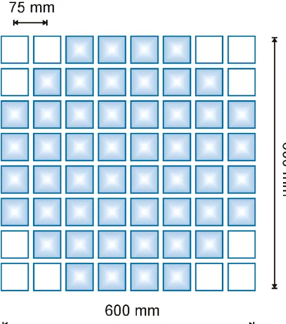
(3) The method The previous article [1] specifies the configuration and the relevant parameters of the antenna used in this work. Table 1 summarizes and lists its parameters. In this table, the reception and transmission modes are denoted as Rx and Tx, respectively. When the antenna is installed on a geostationary satellite, it can generate eight fundamental radiation patterns. These are described as: Rx mode, a global beam to cover a specified zone on the Earth’s surface; one fixed pencil beam, that points to a certain pre-established angular direction; and finally two movable beams with the capability of scanning the complete hemisphere of the earth. The Tx mode uses the same number of beams and specifications as the Rx mode. The coverage zone, that is, the zone of illumination of the global beam of the antenna, is the cone enclosed by the variation of (coordinates spatial angles, with 0   c and 0 2 ( measured from the zenith of the plane of the array). Figure 1 represents antenna dimensions and its active and passive subarrays. It can be seen that 12 elements placed on the vertices of the square were inactivated. For our requirements, a power pattern quasi-null is positioned at pre-established angles (qnqn) inside the coverage zone of the global beam of the antenna, at the center frequency of Rx band. After this, a mapping of 121=11x11 points in the appropriate zone is taken, considering uniformly spaced (u,v) positions, where the transformations: u  sin cos. v  sin sin. (1). replace the () values. The choice of -0.2  u  0.2 and –0.2  v  0.2, includes the () values within the coverage zone..

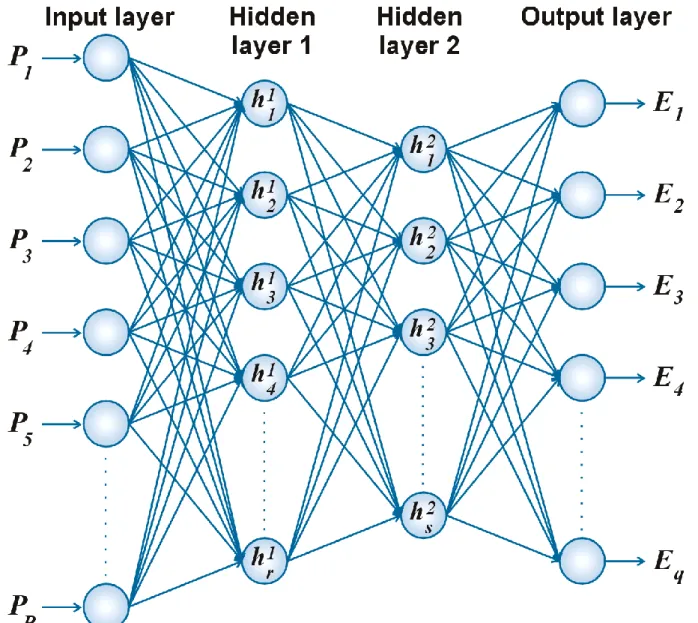
(4) By definition, the synthesis problem in array design consists of finding the excitation distribution of the antenna elements, when a power -or field- pattern, with specified characteristics established by the designer. On the other hand, in the analysis problem, when an excitation distribution is given, the power -or field- pattern is obtained with an empirical or analytical formulation. Subsequently, the synthesis problem can be viewed as the inverse formulation for a certain (previously unknown) excitation distribution. Some authors, as Funahashi [6], have stated that neural networks with non-linear transfer functions can be considered as function universal approximators. Based on these justifications and on their own experience [7-9], a Multilayer Perceptron feed-forward architecture network (MLP) is proposed in this work by the group: Artificial Neural Networks and Adaptive Systems Laboratory2 in order to obtain the excitation distribution of the array when a quasi-null position has been established in its power pattern.. Application For our purpose, a four-layered perceptron gives high-quality results, with the mapping of the power pattern (measured in dB) as input vector, and denoted as Pp (with 1 P  121). The 52-element excitation distribution is separated into real and imaginary parts, as output vector Req, Imq (1 q  52), and two hidden layers: hr1 (1 r  100) and hs2 (1 s  80). The training process of this particular ANN has been performed with 200 pairs of input-output vectors. In the validation process, 25 pairs were used. For better results, two ANN were constructed separately, with their processes of trainingvalidation carried out as follows: on the one hand, an ANN with the PP and Req as input and output vectors, respectively, and, on the other, with PP and Imq as before. Figure 2 gives the schematic of each ANN, with the generic output vector denoted as Eq repre-.

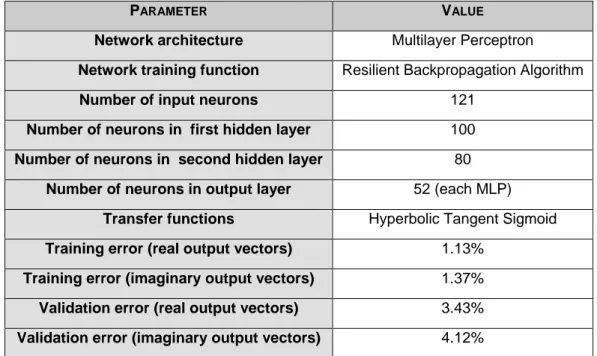
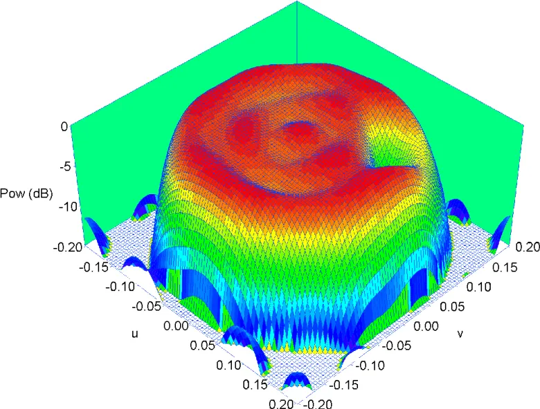
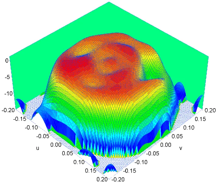
(5) senting the Req or Imq vector, as corresponds. Table 2 summarizes the fundamental characteristics of each ANN, and the errors obtained in their training and validation processes. Figure 3 represents an example of the desired power pattern, with a quasi-null positioned at (uqn = 0.08, vqn = 0.08) and at –10.84 dB below the maximum power. The ripple in the coverage zone is  0.91 dB. Figure 4 represents the ANN response for the same case, after the training process has been completed, with a ripple slightly degraded to  1.15 dB, and the depth of the quasi-null raised at –10.17 dB.. Conclusions The architecture of the multilayer perceptron presented here allows rejection of some interference in the coverage zone of a planar array radiation pattern, when its position has been established. Although the quasi-null positioning was moved within the 0.1  u  0.1 and –0.1  v  0.1 interval, before the training and validation processes, and in order to obtain the 225 pairs of input-output vectors, this must not be seen as a data base itself. The u and v of the equispaced angular points are large enough to admit quasi-null locations between them that change the excitation distribution of the array in a manner that can not be neglected. The training of each network takes about 4 minutes, in a computer with an Athlon XP 1800 processor, running at 1.53 GHz. In the simulation process, after the neural network has been trained, the positioning of the quasi-null in a desired location can be done quickly (less than one second in the same PC), and with high-performance response of the radiation diagram. It can be seen that, as an immediate application, this scope could be expanded through the hardware implementation of the ANN in the array itself. As the ANN presented here represents, in a discretized way, the inverse equation of a radiation pattern of a planar antenna. This technique could be used, in a further in-.

(6) vestigation, to diagnosis array faults by using measured values of its own far-field amplitude [10], its input impedance [11] and / or its mutual coupling [12]. It would be very useful method for antennas permanently or semi-permanently deployed in space, and for any case that requires the use of costly near-field measurement facilities.. References [1]. J. A. Rodríguez, F. Ares, A. G. Pino, and E. Moreno, “Synthesis of a Geostationary Antenna with Eight Independently Variable Beams”, IEEE Antennas and Propagation Magazine. To be published in August, 2002.. [2]. W. H. Press, S. A. Teukolsky, W. T. Vetterling, and B. P. Flannery, “Numerical Recipes in C”, Second Edition, Cambridge University Press, 1992, pp. 444-455.. [3]. A. H. El Zooghby, C. G. Christodoulou, and M. Georgiopoulos, “Performance of Radial-Basis Function Networks for Direction of Arrival Estimation with Antenna Arrays”, IEEE Trans. on Antennas and Propagat., 45, nº 11, 1997, pp. 1611-1617.. [4]. A. H. El Zooghby, H. L. Southall, and C.G. Christodoulou, “Experimental Validation of a Neural Network Direction Finder”, 1999 IEEE Int. Ant. Propagat. Symp. Dig., 37, 1999, pp. 1592 - 1595.. [5]. A. H. El Zooghby, C. G. Christodoulou, and M. Georgiopoulos, “Adaptive Interference Cancellation in Circular Arrays With Radial Basis Function Neural Networks”, 1998 IEEE Int. Ant. Propagat. Symp. Dig., 36, 1998, pp. 203 - 206.. [6]. K. I. Funahashi., “On the Approximate Realization of Continuous Mappings by Neural Network”, Neural Networks, 2, 1989, pp. 183-192..

(7) [7]. M. P. Gómez-Carracedo, J. M. Andrade, E. Fernández, D. Prada, J. Dorado, J. Rabuñal, and A. Pazos, “Clasificación de Refrescos y Zumos Comerciales de Manzana en Función de su Contenido Real de Zumo Mediante Espectroscopia IR. y. Redes. Neuronales”,. XV. Encontro. Galego-Portugués. de. Química, A Coruña, 2001. [8]. J. Dorado, A. Santos, A. Pazos, J. R. Rabuñal, and N. Pereira, ”Training of Recurrent ANN with Time Decreased Activation by GA to the Forecast in Dynamic Problems”, SCI 99/ ISAS 99, Orlando, USA, 1999.. [9]. J. Dorado, A. Santos, A. Pazos, J. R. Rabuñal, and N. Pereira, “Automatic Selection of The Training Set with Genetic Algorithms for Training Artificial Neural Networks”, Genetic and Evolutionary Computation Conference, GECCO 2000, Las Vegas, Nevada, 2000.. [10] J. A. Rodríguez, F. Ares, H. Palacios, and J. Vassal’lo, “Finding Defective Elements in Planar Arrays Using Genetic Algorithms”, Progress in Electromagnetics Research, PIER 29 (Ed. J.A. Kong), EMW Publishing, Chapter 2, Cambridge, MA, USA, 2000, pp. 25-37. [11] J. A. Rodríguez, F. Ares, and E. Moreno, “Waveguide-Fed Longitudinal Slot Array Antennas: Fault Diagnosis Using Measurements of Input Impedance”, Microwave Opt. Technol. Lett., 32, nº 3, 2002, pp. 200-201. [12] H. M. Aumann, A. J. Fenn, and F.G. Willwerth, “Phased Array Antenna Calibration and Pattern Prediction Using Mutual Coupling Measurements”, IEEE Trans. on Antennas and Propagat., 37, nº 7, 1989, pp. 844-850..

(8) TABLES AND FIGURES Table 1. Antenna relevant parameters Active subarrays. 52. Passive subarrays. 12. Number of elements of each subarray. 8. Antenna dimensions. 600 x 600 mm2. Distance between subarrays. 75 mm. Rx Band. 7.90-8.15 (GHz). Tx Band. 7.25-7.50 (GHz). Coverage zone. c = 8.7º (deg). Table 2. Parameters of the two performed MLP and errors obtained in training and validation processes. PARAMETER. VALUE. Network architecture. Multilayer Perceptron. Network training function. Resilient Backpropagation Algorithm. Number of input neurons. 121. Number of neurons in first hidden layer. 100. Number of neurons in second hidden layer. 80. Number of neurons in output layer. 52 (each MLP). Transfer functions. Hyperbolic Tangent Sigmoid. Training error (real output vectors). 1.13%. Training error (imaginary output vectors). 1.37%. Validation error (real output vectors). 3.43%. Validation error (imaginary output vectors). 4.12%.

(9) Figure 1. Antenna spatial configuration. Filled squares represent active subarrays..

(10) Figure 2. Architecture of the MLP feed-forward network used in this work..

(11) Figure 3. Desired power pattern taken with the quasi-null position at (uqn= 0.08,vqn= 0.08) and depressed –10.84 dB below the maximum of the coverage zone. Ripple obtained:  0.91 dB..

(12) Figure 4. Power pattern obtained after the neural network has been trained, corresponding this example to that given in figure 3. Quasi-null depressed –10.17 dB below the maximum. Ripple obtained:  1.15 dB..

(13)