Bursting SN 1996cr's bubble: hydrodynamic and X ray modelling of its circumstellar medium

Texto completo

(1)Mon. Not. R. Astron. Soc. 000, 1–21 (2002). Printed 24 September 2013. (MN LATEX style file v2.2). arXiv:1005.1090v1 [astro-ph.HE] 6 May 2010. Bursting SN 1996cr’s Bubble: Hydrodynamic and X-ray Modeling of its Circumstellar Medium V. V. Dwarkadas,1⋆ D. Dewey,2†F. Bauer3,4,5‡ 1. Department of Astronomy and Astrophysics, U Chicago, 5640 S Ellis Ave, Chicago, IL 60637 Kavli Institute, Massachusetts Institute of Technology, Cambridge, MA 02139 3 Space Science Institute, 4750 Walnut Street, Suite 205, Boulder, Colorado 80301 4 Pontificia Universidad Católica de Chile, Departamento de Astronomı́a y Astrofı́sica, Casilla 306, Santiago 22, Chile 5 Columbia Astrophysics Laboratory, 550 W. 120th St., Columbia University, New York, NY 10027 2 MIT. ABSTRACT. SN1996cr is one of the five closest SNe to explode in the past 30 years. Due to its fortuitous location in the Circinus Galaxy at ∼ 3.7 Mpc, there is a wealth of recently acquired and serendipitous archival data available to piece together its evolution over the past decade, including a recent 485 ks Chandra HETG spectrum. In order to interpret this data, we have explored hydrodynamic simulations, followed by computations of simulated spectra and light curves under non-equilibrium ionization conditions, and directly compared them to the observations. Our simulated spectra manage to fit both the X-ray continuum and lines at 4 epochs satisfactorily, while our computed light curves are in good agreement with additional flux-monitoring data sets. These calculations allow us to infer the nature and structure of the circumstellar medium, the evolution of the SN shock wave, and the abundances of the ejecta and surrounding medium. The data imply that SN 1996cr exploded in a low-density medium before interacting with a dense shell of material about 0.03pc away from the progenitor star. We speculate that the shell could be due to the interaction of a blue supergiant or Wolf-Rayet wind with a previously existing red supergiant (RSG) wind. The shock wave has now exited the shell and is expanding in the medium exterior to it, possibly the undisturbed continuation of the dense RSG wind. The narrow lines that earned SN 1996cr its IIn designation possibly arise from dense, shocked clumps in the CSM. Although the possibility for an LBV progenitor for this Type IIn SN cannot be completely excluded, it is inconsistent with much of the data. These calculations allow us to probe the stellar mass loss in the very last phases (< 104 years) of a massive star’s life (> 106 years) , and provide another means to deducing the progenitor of the SN. Key words: circumstellar matter; methods: numerical; techniques: spectroscopic; supernovae: individual: SN 1996cr; stars: winds, outflows; X-rays: individual: SN 1996cr. 1. INTRODUCTION. Core-collapse supernovae (SNe) arise from stars with zeroage main-sequence masses & 8M⊙ . However, decades of research has failed to determine a direct relationship between the various SNe types (as classified based on their optical spectra and light curves) and the progenitor stars that gave rise to the SNe. It is not clear how the type IIP, IIL, IIb, IIn, Ib and Ic types relate to the properties of their respective progenitor stars. The progenitors themselves, as it turns out, are not very well known, with the. ⋆. E-mail: [email protected] † [email protected] ‡ [email protected]. handful of identified ones appearing to be associated almost exclusively with Type IIP SNe (Smartt 2009). It had been surmised that the main progenitors of core-collapse SNe were red supergiants (RSGs) and Wolf-Rayet (W-R) stars (Falk & Arnett 1977; Podsiadlowski 1992). The explosion of SN 1987A revealed that blue supergiants (BSGs) could also be SN progenitors (Sonneborn et al. 1987), perhaps in a binary system (Morris & Podsiadlowski 2007; Podsiadlowski et al. 2007). In the last decade there has been discussion of LBV stars being the progenitors of Type IIn SNe (Chu et al. 1999; Salamanca 2000; Kotak & Vink 2006; Vink 2008; Smith 2008; Trundle et al. 2008, 2009; Gal-Yam & Leonard 2009), which is problematic because stellar theorists have mainly placed the LBV stage as an intermediate post-main sequence stage, not as a pre-explosion.

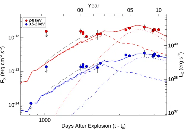
(2) 2. Dwarkadas et al.. phase (Schaller et al. 1992; Langer 1993; Langer et al. 1994; Stothers & Chin 1996; Garcia-Segura et al. 1996; Maeder et al. 2005; Maeder & Meynet 2008). The problem is clear - we rarely know the progenitor star that led to a SN explosion, because it has to be typed from pre-explosion images, leading to significant ambiguity and potential bias. The expansion of the SN shock wave and the resulting emission due to circumstellar interaction (Chevalier & Fransson 1994) opens up another window into the exploration of the pre-SN star. The thermal emission from this interaction, including the X-ray and optical emission, and to some extent the non-thermal radio emission (Chevalier 1982b), depends directly on the external density. Thus an accurate analysis and interpretation of this emission acts as a probe of the density profile. In the case of core-collapse SNe, which lose a significant amount of mass prior to collapse, the surrounding medium is formed by material from the pre-explosion star. Decoding the structure of this circumstellar medium therefore will allow us to probe the mass-loss parameters of the pre-SN star, which can then be linked to the stellar parameters. Thus this provides a way to explore the stellar parameters even after the star ceases to exist, and allows us to probe the pre-SN properties of classes of SN that have heretofore lacked progenitor counterparts. In this paper we pursue this method for the unusual Type IIn SN 1996cr. This SN, which exploded around 1996 but was only discovered about 11 years later, is only the second SN after SN 1987A which shows increasing radio and X-ray emission over a sustained period of a few years (Bauer et al. 2008). Bauer et al. (2008) suggested that the increasing X-ray and radio emission may be associated with a dense shell of material which the expanding SN shock wave interacts with a couple of years after explosion. Herein we carry out hydrodynamical simulations to evaluate this hypothesis, and to decipher the detailed structure of the circumstellar medium into which the shock wave from SN 1996cr is expanding. We compute the X-ray lightcurves and X-ray spectra using non-equilibrium ionization conditions, which we compare with high-resolution Chandra observations. We achieve a detailed agreement which, given that we are using a single model across multiple epochs, affirms the validity of our hydrodynamical model, and allows us to constrain a range of abundances for both the material ejected in the explosion and the surrounding circumstellar medium. The plan of this paper is as follows: In §2 we review the observational details of SN 1996cr, including our recent High Energy Transmission Grating (HETG) spectra which motivated this analysis. §3 describes the reasoning behind our model of the circumstellar medium (CSM), and the results of the hydrodynamical modelling of the SN ejecta interacting with the CSM. Our techniques for computation of the X-ray light curves and spectra from the hydrodynamical models, and the resultant X-ray emission, are outlined in §4. §5 puts the narrow lines that earned SN 1996cr its Type IIn designation into the context of the overall model. In §6, the implications for the progenitor, and the abundance determinations, are discussed in depth. Finally, §7 summarizes our results and outlines future work in this area.. 2. SN 1996CR. This luminous type IIn SN was only identified in the nearby Circinus Galaxy (3.7±0.3 Mpc; Koribalski et al. 2004) ∼11 years after it was believed to have exploded (Bauer 2007; Bauer et al. 2008), but its remarkable evolution was fortuitously captured in archival data from HST, Chandra, XMMNewton, Spitzer, and several ground-based optical and radio observatories taken for other purposes. Initially undetected at radio and X-ray wavelengths, the SN emission jumped by a factor of at least ∼ 300 at radio wavelengths about 2 yrs after explosion. It continued to increase modestly for 8 years before finally exhibiting signs of a potential X-ray and radio turnover in late 2008. Fig. 1 shows the radio and X-ray evolution of SN 1996cr. Unfortunately, only upper limits exist for the first few years after the explosion. But even these are sufficient to illustrate the low level of emission in the initial years, followed by a steep rise in the radio, and a less steep but no less significant rise in the X-ray emission, which lasted for roughly a decade. This behavior is reminiscent of the more famous SN 1987A, whose emission follows a similar pattern (McCray 2003, 2007), albeit with a factor of ∼ 1000 lower luminosity (Bauer et al. 2008). Emission from SN 1987A was explained by Chevalier & Dwarkadas (1995) as arising from the interaction of the SN shock wave with a dense HII region interior to the circumstellar ring seen in the equatorial region. Further interaction with the denser ring should result in a continuously increasing light curve in the case of SN 1987A (Dwarkadas 2007b). Early (2004) HETG X-ray data of SN 1996cr showed hints of the complex velocity structure, similar to that seen in the optical. This, coupled with the similarity with SN 1987A and the need to investigate such an unusual SN further, motivated a deep 485ks Chandra HETG observation of SN 1996cr in early 2009, with regular monitoring thereafter. A companion paper (Bauer et al. 2010, in preparation) describes the analysis of the HETG spectrum. In this paper we concentrate on the interpretation of the X-ray emission, and the computation of the structure of the medium into which the SN shock wave is expanding. The steep rise in the Xray and radio, and the more recent turnover in the emission (see Fig. 1) point to an interaction of the SN shock wave with high density material, from which the shock wave has now emerged. This possibility was already indicated by an analysis of the radio spectrum earlier in Bauer et al. (2008). Herein we provide a more quantitative assessment of the various properties of the circumstellar medium based on the X-ray data. The 2009 HETG spectrum (shown later in Fig. 6) is probably one of the most detailed X-ray spectra of a young supernova, next only to SN 1987A. The well-resolved emission lines allow us to estimate the relative abundances of the ejecta to reasonable accuracy. Combined with lower signalto-noise HETG spectra from Chandra in 2000 and 2004, and a high signal-to-noise XMM-Newton p-n spectrum in 2001, as well as other CCD-quality X-ray data, it provides a strong basis for accurate comparison of our simulated spectra with the observations, allowing us to fine tune our models. Any model of the medium into which SN 1996cr is expanding must be able to explain the increase in the radio and X-ray lightcurves, and the spectral details. The model that.

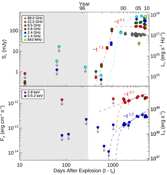
(3) Hydrodynamics and X-Ray Emission from SN 1996cr. Year 96. 1028. 89.0 GHz 22.5 GHz 8.5 GHz 4.8 GHz 2.4 GHz 1.4 GHz 843 MHz. Lν (erg s-1 Hz-1). ~t-0.1 1027. ~t 7.3. 10. 1026. 1. 1025 2-8 keV 0.5-2 keV. FX (erg cm-2 s-1). 05 10. ~t 0.7. 10-12 1039. ~t 1.2 10-13. LX (erg s-1). Sν (mJy). 100. 00. 3. 1038. 10-14 1037 10. 100 1000 Days After Explosion (t - t0). Figure 1. (Top) The radio light curve of SN 1996cr. All available data from 843 MHz to 89 GHz are shown (some of which is previously unpublished and will be presented in Bauer et al., in preparation). Only upper limits are available during the first 3 years. The radio flux clearly shows a sharp increase starting from around 700 days, a flattening of the light curve around 2000 days, and a decrease and turnover around 5000 days. On top of this luminosity evolution in the 8.5GHz band, we see a gradual decreasing absorption at lower frequencies (1.4GHz) that leads to a smoother transition between 1000-3000 days. (Bottom) The X-ray light curve of SN 1996cr over time. Unlike the radio, once detected the X-rays show a more-or-less constant increase over time, and no flattening. However the late-time turnover is present in the X-ray emission also. The upper limits in the first 3 years are quite high, with the points around 700 and 900 days being the most constraining. Sample power-law fits to the light curves are also shown. The simulations in this paper are geared towards explaining the X-ray emission, while being consistent with the radio behavior.. we put forth in this paper is constrained by the following observational parameters: (1) The range of explosion dates, from March 1995 to March 1996 (see Bauer et al. 2008). (2) Observed X-ray upper limits prior to year 2000 and detected fluxes thereafter (Figure 1). (3) A radio VLBI measurement that provides a size measurement, which we take to be the radius of the outer shock. This gives the radius of the outer shock as about 2.8 ×1017 cm at 12 years (with a statistical error of ≈ 20%). (4) Emission-line velocities seen in the X-ray and optical spectra, ranging from 2000-5000 km s−1 . (5) Fits to the temperature (kT) and the absorption column. density at various times, obtained from the X-ray spectra at several epochs. (6) Fits to prominent lines seen in the emission spectra, which constrain CSM and ejecta abundances. (7) The radio light curve (Figure 1).. 3. EJECTA AND CSM MODELS AND HYDRODYNAMICAL CALCULATIONS. In order to study the interaction of the SN ejecta with the surrounding circumstellar medium, we need to delineate the density profile of the ejecta as well as the surrounding.

(4) 4. Dwarkadas et al.. medium. In this first paper we make the assumption that the density structure, of both the ejected material and the surrounding medium, is spherically symmetric, and therefore that a one-dimensional (1D) model will suffice. Although the complexity of line emission seen, especially in the optical spectrum, may indicate otherwise, a spherically symmetric model is a reasonable starting point, given the lack of any imaging constraints. The validity of such an assumption can only be determined by computation of the light curves and spectra resulting from these calculations. As we shall show later, the spherically symmetric assumption appears to be adequate in this regard. The companion paper by Bauer et al (2010) will explore the line shapes and emission in detail for deviations from spherical symmetry. This work will then serve as a launching pad for more complicated explorations of the density structure. Following the work of Chevalier (1982a) and Chevalier & Fransson (1994), we denote the ejecta density dropping off as a power-law with radius (or velocity). Matzner & McKee (1999) narrows this power-law to a value of around 9 or 10; in the current work we adopt a value of 9. In order to conserve mass and energy, the power-law density profile cannot extend all the way to the origin, therefore below a certain velocity the density is assumed to remain constant. This ejecta profile model therefore has two free parameters - the normalization of the outer density profile and the transition-to-plateau velocity; alternatively, these two parameters can be expressed in terms of the ejecta energy and mass. Note that for early times, until the reverse shock reaches the plateau region, only the single parameter of the density normalization is involved in the hydrodynamics and there is a degeneracy between ejecta mass and energy. In this case one can set the energy to a canonical value and use the ejecta mass as the free parameter. Changing the explosion energy scales this mass accordingly (Chevalier & Fransson 1994). Our late time modeling of SN 1996cr shows that in order to match the light curve, the reverse shock must have passed into the plateau region. Fitting the X-ray spectra constrains the ejecta energy and mass to be 1051 ergs and 4.45 M⊙ . The latter mass value is very reasonable for the total ejected material in a core-collapse explosion (Woosley et al. 2002). We note that this gives a characteristic velocity vα = 2 × Ekin /Mejecta = 4740 km s−1 which is suggestive of a stripped envelope SN (Maurer et al. 2009). In §6.1 we will discuss the connection with stripped envelope SNe in more detail.. model (Chevalier 1982a) for SN evolution. Detailed results for the X-ray emission using the self-similar model, for various values of the parameters mentioned below, and investigating several different assumptions for the forward and reverse shocks, are given in Fransson et al. (1996). Herein we present a simplified analysis that encapsulates the important ideas relevant to this work. The X-ray luminosity Lx from a source depends on the electron density ne , the emitting volume V and the cooling function Λ Lx ∼ ne 2 Λ V. (1). We assume that the density of the medium into which the SN shock wave is expanding goes as r −s . The emission arises from a thin shell of radius ∆r at a mean radius r , whose volume V can be expressed as 4πr 2 ∆r. Note that for self-similar evolution, ∆r ∝ r, and therefore V ∝ r 3 . For a SN in the early stages, the temperature is going to be much larger than 107 K, and the cooling function is assumed to vary as T 0.5 (Chevalier & Fransson 1994). For a strong shock, T ∝ vs 2 , and therefore the cooling function Λ ∝ vs ∝ r/t in the self-similar case. Therefore we get Lx ∼ r −2s. r 3 r t. (2). which gives Lx ∼. r 4−2s t. (3). CSM Density Profile -Power-Law Model. For s=2, a SN expanding in a wind with constant massloss parameters, this gives the well-known result that the emission decreases inversely with time, Lx ∝ t−1 . For s=1, we get Lx ∝ r 2 /t. In the self-similar case, r ∝ tα , and therefore we get that Lx ∝ t2α−1 . The parameter α = (n − 3)/(n − 1) for s=1 with ρSN = At−3 v −n (Chevalier 1982a), which is greater than 0.5 for all n > 5. Therefore 2α − 1 > 0, and the power-law exponent is always positive, leading to an X-ray evolution that increases with time, even though the density is decreasing as r−1 . For s=0, Lx ∝ t4α−1 . With α > 0.4, (0.4 being the value it would have in the Sedov-Taylor stage), the X-ray luminosity increases with time for all values of α. Theoretically, it is therefore possible to envision an increasing X-ray luminosity with a CSM whose density is constant or even decreasing with radius. The radius can then be expressed in terms of the self-similar solution. We use the self-similar solution to show that this approximation is not a good one in the current situation, for the following reasons:. Elucidation of the density structure of the CSM required considerable trial and error. The simplest assumption of a CSM is one with a power-law density profile r−s , where s = 0 for a constant density medium and s = 2 for a wind. A wind whose mass-loss parameters are changing with time can result in other values of s. Therefore we first explored the validity of such monotonic-with-radius models. The light curve indicates that the X-ray emission began increasing linearly about two years after explosion. In theory it is possible to have the X-ray emission increasing with time even if the ambient density is decreasing with radius. This can be shown in the context of the self-similar. (i) The radio spectra indicate that the absorption was high even two years after explosion (Bauer et al. 2008), and that as the SN shock expanded within this region the freefree absorption continually decreased. This suggests a region of high absorption into which the shock was expanding two years after the explosion. The absorption decreased as the shock made its way through this region. It would be difficult to explain this with a constant or continually decreasing density profile. (ii) In the discussion above the post-shock temperature is related to the shock velocity, which varies as vs ∝ tα−1 . Thus the temperature will vary as T ∝ t2α−2 . For example,. 3.1.

(5) Hydrodynamics and X-Ray Emission from SN 1996cr in order to get an X-ray luminosity Lx ∝ t1.0 , roughly intermediate between the hard and soft luminosity slopes seen in Figure 1 , we can take s = 0.6 and n = 9. Then α = 0.7142, and Lx ∝ t1.0 from equation 3. This would mean that the temperature would vary as t−0.57 , which equates to an expected temperature drop of 1.7 between 2000 and 2009. Such a temperature variation is not seen. Instead the X-ray data (Bauer et al. 2010) above 2 keV show little spectral variation, and hence little apparent temperature evolution, over 9 years. The spectrum below 2 keV does vary somewhat, although it is not clear whether this is because of decreasing absorption in the soft X-ray regime or whether it is because the spectrum is actually becoming softer. (iii) A radius of 2.8e17 at a time of 12 years implies an average velocity of 7500 km s−1 . The optical and X-ray spectra do not show velocities exceeding 5000 km s−1 , and in most cases somewhat lower. If we assume spherical symmetry and an average velocity of 4000 km s−1 from 2000 to 2008 (when spectra are available) then it suggests that the average velocity in the first 4-5 years (depending on explosion date) must have exceeded an average velocity of 12,000 km s−1 . A power law model has shock velocity varying as vs ∝ tα−1 , which would make it extremely difficult, if not impossible, to fit such a velocity profile for reasonable values of α. Whereas a model with a lower CSM density early on and a higher density later could fit it easily. Using our earlier example, we can construct a model with n = 9 and s = 0.6 using the self-similar solution, which satisfies the constraint that the shock radius be 2.8e17 at 12 years. This model gives a velocity of 5290 km s−1 at 12 years. While this is somewhat high, it could be considered acceptable within the error bounds. However such a model would also predict a velocity of almost 6000 km s−1 at 8 years and 6450 km s−1 at 6 years, which is not supported by the observations. Note that a constant density model with n=9 would have vs ∝ t−0.33 , which would make this discrepancy worse. (iv) In a model with monotonically decreasing density, the density of the CSM would need to be significantly high throughout the evolution for the shock velocity to decelerate to a few thousand km s−1 in a few years, as suggested by the X-ray and optical spectra. For instance, in the above model with n = 9 and s = 0.6, the density at 5 ×1016 cm would be 7.71e-21 g cm−3 . This is about 3800 times greater than what is in our simulations presented in the next section, which would result in the X-ray emission, especially the hard X-rays, being about 107 times greater on average, significantly exceeding the upper limits derived from archival observations. (v) The radio emission is increasing significantly with time after about 2 years (Figure 1), which is hard to accomplish in a model with decreasing density. In particular free-free absorption by itself cannot account for this increase (Bauer et al. 2008), there still needs to be a flux increase > 100. This can best be implemented with a density increase, as the radio emission, although non-thermal, indirectly depends on the external density (Chevalier 1996). (vi) The X-ray emission increases significantly after two years. A simple power-law increase in the X-ray flux, as predicted by the self-similar model, cannot match the data, which requires at least two distinct power-laws, with the upward slope becoming much steeper after 2 years. This would then require at least two different density slopes, with the. 5. density decreasing slower in the second case. When combined with the VLBI radius constraint, and the velocity and temperature constraints outlined above, it would be almost impossible to make the power-law model consistent with all the available data. The above arguments suggest that a CSM density profile that shows a simple power-law decrease would not work. Although a self-similar solution is not applicable, many of the same arguments can be used to show that an increasing power-law density profile from the origin (the stellar surface) also would not work. Instead, a density profile where the density changes after 2 years is suggested.. 3.2. CSM Density Profile - High Density Shell. The above discussion clearly argues for these basic requirements of any CSM model for SN 1996cr: a CSM whose density is low close to the star, then increases sharply with radius. This would fulfill both the velocity and density criteria outlined above, as well as lead naturally to the observed radio spectra and light curves. One way to arrive at such a distribution is with a low density wind medium followed by a thin, dense shell, as is often seen around massive stars (Weaver et al. 1977; Chu 2003; Cappa et al. 2003; Chu 2008), and in the nebula around SN 1987A (Blondin & Lundqvist 1993). In this paper we consider such a distribution. The inner and outer radius of this shell, the shell density, and refinement of the CSM density structure, are obtained via an iterative procedure that consisted of adopting a value for the shell parameters, computing the hydrodynamic interaction, calculating the X-ray light curves and spectra, and re-iterating until a reasonable fit was obtained between the simulated and observed spectra and light-curves. This took on the order of a dozen iterations before convergence was obtained. The model that we finally converged on has a shell with density around 1.28 ×10−19 g cm−3 extending from 1 ×1017 to 1.5 ×1017 cm. The X-ray light curves and spectra are highly sensitive to the shell parameters, i.e. the inner and outer shell radii and shell density, and so manage to constrain them quite tightly. Even a 20% deviation of the shell radii from these values destroys the agreement with the lightcurve, while a factor of 1.3 in the density has about the same effect. Therefore the shell itself is strongly constrained by the X-ray data. A rearrangement of the mass in the shell, i.e. a modest change in the density profile that does not alter the total mass (Figure 2), can result in modest changes to the early-time X-ray flux, as shown in Figure 5. For the CSM inside of the shell, we have assumed a structure resemblant of a wind-blown bubble, with an initial freely expanding wind whose density drops as r−2 ending in a wind termination shock, which is assumed to be a strong shock. Beyond this is a constant density shocked wind region. The wind density, and location of the wind termination shock, are constrained only by the density of the shocked wind region, and are obtained as described in the Appendix. For the standard case described here and shown in Figure 2, the value of the wind parameter Ṁ /vw is 6.76 ×1011 g cm−1 , the wind termination shock is located at 1.63 ×1016 cm, and the shocked wind region has a constant density of 8.15 ×10−22 g cm−3 ..

(6) 6. Dwarkadas et al.. The structure of the medium beyond the dense shell is difficult to estimate properly, since the shock front has not had much time to expand within it. One assumption is that the dense shell consists of fully swept-up wind material. In this case the CSM density structure resembles a wind-blown bubble formed by the interaction of a supersonic wind with the slower wind from a previous epoch; the dense shell is composed entirely of the slower wind material that has been swept-up. The mass of the shell must equal the total wind mass up to the outer radius of the shell, or Mshell = (Ṁw /Vw ) Rshell , where the subscript w refers to the outer wind. Since the shell outer radius is known, and the mass is defined once we have the shell boundaries and shell density, this provides us with the wind parameters Ṁw /Vw . Assuming constant wind parameters, the density of the material outside the shell at any given radius r can then be expressed as that of a freely expanding wind ρ = Ṁw /Vw ×1/(4πr 2 ). This was one of the two assumptions that we have tried, and since it gives satisfactory results over the short period of time that the shock is interacting with this region, we have continued to use it. (The other assumption involved a constant density profile exterior to the shell. However in that case the shell mass was always found to be larger than the mass of the swept-up material given that density, suggesting a complicated origin for the shell. A constant density profile either gives too small a density close in or too large a density further out, depending on its magnitude. Furthermore, the total absorption column from any constant density profile that provides adequate X-ray emission beyond the dense shell increases too fast, and thus such a profile cannot be sustained beyond 0.4pc in any reasonable model. Since the wind profile anyway fits better, we did not explore the constant density assumption further). The final density profile for the SN ejecta and CSM that we have used, which forms the initial conditions for the hydrodynamical simulations, is shown in Fig. 2. The thin solid lines superimposed on the constant density shell are intended to show how rearranging the mass to perturb the density in this fashion can lead to a modest change in the X-ray lightcurve (the dashed gray line in Figure 5).. 3.3. Hydrodynamic Simulations. We carried out hydrodynamical simulations to compute the interaction of the SN ejecta with the CSM. The simulations were carried out using VH-1, a three-dimensional finite-difference hydrodynamic code based on the Piecewise Parabolic Method of Colella & Woodward (1984). Although cooling is included in these simulations via the inclusion of a cooling function, it was not found to play an important role in the 1D calculations. However the cooling time of the shock within the shell was of the same order of magnitude as the evolution time, and it is possible that in multi-dimensional calculations, where the growth of instabilities can give rise to dense clumps, cooling could prove to be more effective1 .. 1 Our X-ray spectral calculation, as well as the formation of narrow optical lines, does in fact require the presence of dense clumps, but they comprise at most 1% of the mass. In these scenarios cooling is important, and in fact the shock within the clumps is assumed to be radiative in order to account for the narrow-line. The simulation was started with the initial conditions described above, and the SN ejecta allowed to expand into the surrounding medium. The evolution of the various dynamical and kinematic quantities over time are shown in Fig. 3. The SN ejecta expand quickly in the low density medium (see Fig. 4) until they reach the higher density shell in about 20 months. The shock, which was expanding very rapidly up to this time, is instantaneously decelerated by the high density, and its velocity drops to about 2000 km s−1 due to the high pressure. As seen in Fig. 3, the high pressure region between the forward and reverse shocks gets highly compressed. The collision of the ejecta with the high density shell sends a lower velocity transmitted shock into the dense shell, and a reflected shock is formed that travels back into the ejecta. The reflected shock quickly overtakes the original reverse shock, thus thermalizing the ejecta faster than the SN shock itself would have done. The transmitted shock gradually increases in velocity as the highly over-pressured region slowly depressurizes, and then attains a more or less uniform velocity of around 5500 km s−1 . The interaction of the shock wave with the high density shell lasts for about 4.6 years (from t ∼ 1.5 to t ∼ 6.1 years.). The structure of the interaction region resembles the interaction of a power-law profile with a constant density medium, as expected, and the density decreases from the reflected shock to the contact discontinuity. Since the pressure does not vary much, the temperature is almost inversely proportional to the density, and increases outwards from the reflected shock, until it reaches a large value at the contact discontinuity. We note that the structure is comparable to that described by the self-similar solution for a steep ejecta density profile colliding with a wall (Chevalier & Liang 1989). The comparison is close but not exact, since the shock in this case imparts some motion to the shell, which is not included in Chevalier & Liang (1989). It is also interesting to note that, given the presence of the dense shell so close to the star, the density into which the forward shock is propagating, while in the shell, is much higher than the density into which the reverse shock is propagating. This is contrary to a general expansion in a power-law or constant density medium, and results in the temperature behind the forward shock (∼ 108 ) being initially lower than the temperature behind the reverse shock (∼ 109 ). Therefore we expect that the major contribution to the X-ray emission in the 0.5-10 KeV wavebands at this early time arises from the shocked circumstellar material. As the shock continues to expand, the temperature behind the forward shock increases, whereas that behind the reverse shock decreases as the shock expands into the increasing steep power-law ejecta density profile. When the transmitted shock exits the shell and begins to reform in the freely expanding wind around it, the reflected shock is then interacting with the constant density ejecta, whose density is higher than that of the wind medium. The density behind the reflected shock is higher than that behind the forward shock, its temperature lower, and the emission emission. However this would affect only a small portion of the material. In any case, these clumps are not included in the spherically symmetric numerical hydrodynamics simulations, and they would not affect the general hydrodynamical evolution described herein..

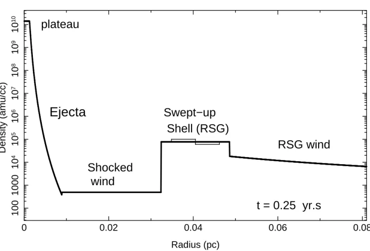
(7) Density (amu/cc) 100 1000 104 105 106 107 108 109 1010. Hydrodynamics and X-Ray Emission from SN 1996cr. 7. plateau. Ejecta. Swept−up Shell (RSG) RSG wind Shocked wind t = 0.25 yr.s. 0. 0.02. 0.04. 0.06. 0.08. Radius (pc) Figure 2. The initial density profile of the SN ejecta and CSM, used as initial conditions in the hydrodynamic simulations. Starting from left and moving outwards in radius, the density profile shows the constant density plateau region of the SN ejecta, followed by the steeply decreasing ejecta profile which goes as r−9 . Beyond this is the circumstellar medium. The ejecta have already crossed the freely expanding wind region (not shown). Going outwards in radius, we encounter a uniform density shocked-wind region, the high density shell, and the freely expanding outer wind. A suitable temperature was assigned to each component. The pressure (and temperature) that we use for the initial conditions is not important, since it is significantly smaller than the pressure of the gas shocked by the SN blast wave. The labels attributed to the various sections of the CSM reflect the discussion in §6. The thin solid is intended to show how a rearrangement of the mass in the shell in this fashion, without changing any other parameters, can lead to a modest increase in the light curve at early times (< 3 years), shown as the dotted line in Figure 5.. becomes dominated by the reverse shocked ejecta. It was found that a good fit to the late-time emission required that the reverse shock enter the plateau ejecta region. The location of the plateau, the velocity below which the ejecta density remains constant, was adjusted to match the observations, fixing the total ejected mass to the value given in the previous section. Once the transmitted shock exits the shell, it is expanding in the lower density wind, whose density decreases as r−2 . The radius of the forward shock at ≈ 12 years is consistent with that obtained from VLBI imaging to within 5%. Thus this approximation has proved suitable so far, but only time and future data can confirm whether this approximation is valid for the further expansion of the shock wave. While most of the X-ray emission at this point is expected to arrive from the reverse shocked ejecta, the radius and velocity of the forward shock, and therefore the size of the remnant, are determined by the interaction with this wind. It is interesting to note that although the shock is interacting with an r−2 wind, the shock structure is resemblant of the shock interacting with a constant density medium. This is to be expected as it will take a few dynamical times. for the shock to reach the self-similar solution in the wind (Dwarkadas 2005). Over time therefore the entire density structure of the shocked interaction region is predicted to change, with the density at the contact discontinuity going from relatively small to relatively large values. Such a change should be reflected in the X-ray emission over the next few decades.. 4 4.1. COMPUTATION OF THE X-RAY EMISSION AND COMPARISON WITH OBSERVATIONS Non-equilibrium Ionization and Lagrangian Shells. Our goal is to compute the X-ray emission from the output of the hydrodynamic simulation efficiently and with reasonable accuracy. Plasma that has been recently shocked and whose density is low is presumably not in ionization equilibrium (Hamilton et al. 1983; Borkowski 2000; Borkowski et al. 2001); as a rule of thumb this is the case if τ ≡ ne t < 1012 s cm−3 where ne is the electron density and t is the time since the plasma was shocked. Since the.

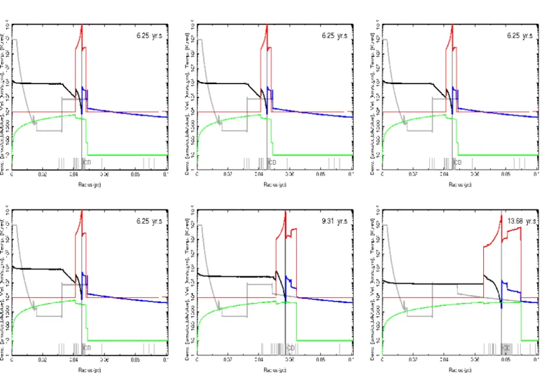
(8) 8. Dwarkadas et al.. Figure 3. These panels depict the hydrodynamic evolution of various quantities: ejecta density (black); CSM density (blue); temperature (red); and fluid velocity (green). The grey vertical lines denote the borders of the mass-shells into which the domain is divided up, for the purpose of computing and tracking the fluid history. The thick grey line shows the initial density profile to enable the reader to see how it changes with time. The last four panels approximate the times when the spectra outlined in §4 were taken. The various panels show, from left to right and top to bottom (1) the initial interaction of the SN ejecta with the shocked wind, and the formation of a forward and reverse shock (2) The interaction with the dense shell, the compression of the interaction region between the shocks, and the formation of a resultant transmitted and reflected shock (3) (HETG-00) The transmitted shock is advancing slowly through the shell, while the reflected shock goes up the steep ejecta incline. Note that the interaction region is slowly growing bigger. (4) (XMM-01) The forward shock has reached the edge of the shell, and will soon start to expand out into the external wind. (5) (HETG-04) The reflected shock reaches the constant density plateau region of the ejecta. Beyond this point, the solution is no longer self-similar, if it indeed ever was given the various transitions. (6) (HETG-09) The evolution of the forward shock in the external wind, while the reverse shock is expanding back into the ejecta plateau region.. plasma impacted by the SN shock wave has a density typically less than 105 cm−3 , the time to reach ionization equilibrium is measured in years and the X-ray emission must be computed using non-equilibrium ionization (NEI) conditions. In general this is done by calculating the evolution of ion fractions using ionization and recombination rates under appropriate simplifying assumptions (Hamilton et al. 1983; Borkowski et al. 1994). Here, however, our approach is to make use of existing NEI codes and appropriately interface them to the hydrodynamics output. We use NEI emission models available in the XSPEC package, vgnei and vpshock, along with “NEI version 2.0” atomic data from ATOMDB (Smith et al. 2001) which has been updated to include relevant inner-shell processes2 . These 2. Files provided by K. Borkowski and http://space.mit.edu/home/dd/Borkowski/. online. at. codes encode the NEI state with only a few parameters; we have chosen to sacrifice some accuracy for speed and simplicity. To calculate the X-ray emission from an individual fluid element these models need information that is based on the R element’s history, in particular the ionization age, τ = ne (t) dt, the current electron temperature, Te , Rand the ionization-age-averaged temperature, < kTe >= Te (t)ne (t) dt/τ (Borkowski et al. 2001). These quantities can be calculated from the set of simulation time steps provided the location of a given fluid element can be determined and followed in time. To this end we regroup the Eulerian output at each time step in a Lagrangian manner, using cumulative mass as the Lagrangian parameter to define and track a set of mass intervals, representing “shells” in 3-D. These mass shells, of order 50 of them, are not as finely spaced as the hydro radial bins (thousands), so we calculate shell-averaged hydrodynamic fluid parameters: pressure pj ,.

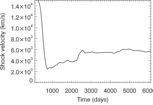
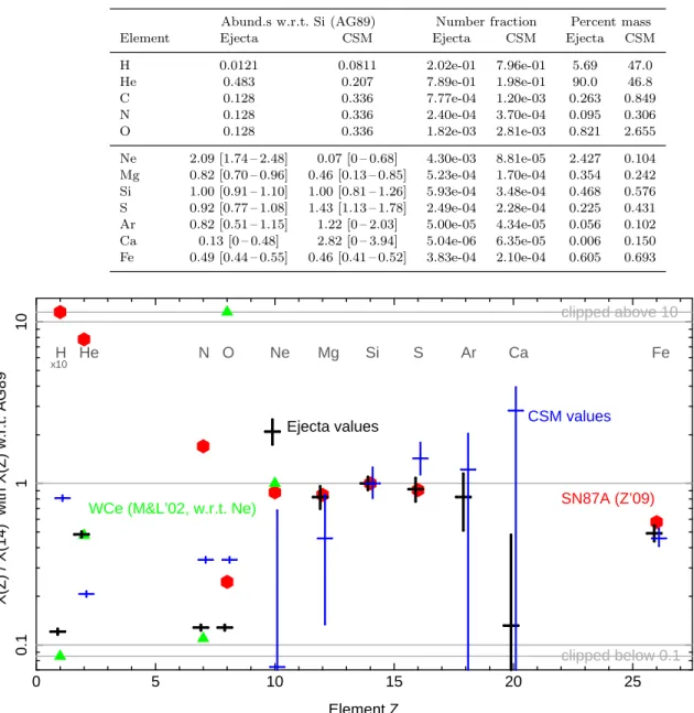
(9) Hydrodynamics and X-Ray Emission from SN 1996cr. 9. Figure 4. The velocity of the SN forward shock during the evolution. It is extremely high (exceeding 20,0000 km/s) in the first few months, but then drops dramatically when the shock encounters the higher density shell, and the interaction region is highly compressed. As the compressed region slowly expands, the velocity rises again as the built-up pressure is released (A similar effect was observed in SN 1987A). After about 6 years, the shock exits the shell, and the velocity increases as it encounters a lower-density medium. As the density profile of the shocked interaction region changes from that in a constant-density medium to that in a wind medium, the velocity remains more-or-less constant, at a velocity around 5500 km s−1 .. density ρj , and radial velocity vj , for each shell at the time steps, tj .. 4.2. Abundances, µ, and Te. The hydrodynamic variables are converted to values relevant for the X-ray emission, ne , Te , through the abundances and the related mean mass per particle, µ. We assign an abundance to each shell of material: shells interior to the contact discontinuity are assigned ejecta abundances and those exterior are CSM. It is possible (and as we argue in the discussion section, most likely) that the CSM can be divided into two phases, the portion interior to the shell and the portion including the shell and exterior to it. However the evolution of the SN ejecta into the region interior to the shell is not constrained by the data. Therefore a single set of abundances is assumed for the CSM for simplicity. It is likely that the ejecta may be layered, as is expected for a massive star, and different abundance distributions should be expected for different layers. However, we have no a priori indication of any of the abundance distribution, and 4 spectra of different resolution spread over 9 years, only the last two of which are actually tracking reverse-shocked emission according to our calculations, would be unable to distinguish between abundances of various layers. Therefore as a first approximation we have considered a single set of ejecta abundances, although our code is easily capable of assigning a unique abundance to each shell of material if required. Define X(Z) as the relative abundance values with re-. spect to a reference number-ratio abundance set, AAG89 (Z); here we use the Anders & Grevesse (1989) abundance set. The mean atomic weight can be calculated as:. P mZ X(Z) AAG89 (Z) Z µA = P Z. X(Z) AAG89 (Z). (4). where mZ is the mass of an ion of element Z. Similarly the mean charge state averaged over all ions is given by: qA =. P. Z. QZ (TCIE ) X(Z) AAG89 (Z) P X(Z) AAG89 (Z) Z. (5). where QZ (TCIE ) gives the average charge state of ion Z, i.e., the average number of free electrons per Z-ion, and TCIE refers to the temperature in collisional ionization equilibrium. This value changes with progressive ionization, however it is dominated by the low-Z elements which are quickly ionized, so we approximate its value based on ionization equilibrium at a fixed temperature, TCIE = 107 K. The mean mass per particle is then: µA µ= (6) 1 + qA where µ here has units of mass. 3 The densities of electrons and ions can now be obtained from the fluid density as:. 3 Note that it is common to informally express µ in implied atomic mass units, µ/mamu , e.g., “µ = 0.5 for a fully ionized H plasma”..

(10) 10. Dwarkadas et al.. ne = qA ρ/µA , ni P = ρ/µA and for a specific ion: nZ = ni X(Z) AAG89 (Z) / Z X(Z) AAG89 (Z). We can now compute the average particle temperature in an element of plasma from the hydrodynamic pressure and density: kThydro = µp/ρ. Since the shocks are collisionless, most of the post-shock energy is transferred to ions, and the electron temperature is generally a fraction β of the ion temperature (Ghavamian et al. 2007). This is accounted for by setting Te = βsh (vsh ) Thydro with the −2 βsh value set to be ∝ vsh as given in Ghavamian et al. (2007); the shock velocity is calculated self-consistently from kThydro = (3/16)µ vsh 2 . Other choices for βsh (vsh ) can be easily implemented if desired. For example, we clipped β to have a minimum value of 0.05 as an approximation to the results of van Adelsberg et al. (2008); however, this produced no significant changes in our calculated flux or spectra as the β values of the mass-cuts are generally well above 0.1. Finally, the β value is modified to include its evolution due to Coulomb interactions: Te /Thydro approaches 1.0 as the ionization age approaches τequil (vsh ). The dependence on shock velocity is given roughly by: τequil ∼ 1010 (vsh /v400 )3 , with v400 = 4×107 cm s−1 ; this follows from the T 3/2 variation of the Coulomb equilibration time constant. For smaller values of τ , β changes such that β ∼ (τ /τequil )0.44 , e.g., as seen in Figure 4 of Michael et al. (2002). With these relations the value of β is increased from its initial post-shock value when the τ of the mass-cut increases sufficiently. 4.3. Implementation and Embellishments. Using the above equations, for each shell at each time step we can calculate the input values needed for the vgnei model (Borkowski et al. 2001): kT, Tau, <kT>, and the norm = 10−14 ∆V ne nH /(4πd2 ), with ∆V the shell volume and d the source distance. The vgnei abundance values are the appropriate set (ejecta, CSM) scaled so that the H abundance is 1. The calculations, from reading the hydro output files to evaluating the XSPEC spectral model, are all done with custom routines written in S-Lang, the interactive scripting language used in the ISIS package (Houck & Denicola 2000). The flexibility of the code also allows us to implement additional modifications to improve the fidelity of the emission calculation as needed. For most mass shells we use the vgnei model with an appropriate τ value based on the shell history as described above. For the case where a mass shell is partially shocked, the shock front is within the shell and a constant τ value is not appropriate since there is a range of τ starting at τ = 0 up to a maximum value. In this case we can calculate the shell’s emission using the vpshock model, which allows us to set a range of τ from a low (zero) to a high value. Inclusion of these partially-shocked shells adds some line emission of lower ion states and smoothes the light curves. There are indications that the X-ray emission from SN 1996cr is not simply the sum of optically thin components: the as-fit NH decreases with observation epoch and the Xray line shapes at high-resolution are asymmetric. These data are examined in more detail in the companion paper (Bauer et al. 2010, in preparation) but the methods to include them in the emission model are briefly summarized here. To self-consistently model the NH effect, we can add. “internal absorption” proportional to the amount of unshocked CSM material external to the forward shock. In the case of the asymmetric line shapes it seems likely, and our hydro model predicts, that there is substantial opacity through the SN ejecta core. Hence some of the redside emission is obscured producing asymmetric lines and reducing the observed flux. Based on simple 3D modeling (Dewey & Noble 2009), a value of 0.75 has been used to account for the amount of flux typically obscured by the core, and a blue-shift and Doppler Gaussian broadening, proportional to the hydro shell velocity, are applied as a first approximation to the line shape from the shell. 4.4. Comparison with the Data. As the previous sections imply, the X-ray emission from a given hydro simulation depends on some additional parameters and assumptions. Perhaps the most influential of these are the elemental abundances assigned to the hydro plasmas. These abundances show up in two main ways: i) they determine the µ value of the plasma and hence affect the electron temperature and the number of electrons per ion (section 4.2), and ii) the abundances of the higher Z elements are responsible for the X-ray emission lines in the spectra. Because we use the XSPEC vgnei (vpshock) routine, the abundances of the 13 elements currently treated by that model are the ones relevant here: H, He, C, N, O, Ne, Mg, Si, S, Ar, Ca, Fe, Ni. These abundances are specified relative to the Anders & Grevesse (1989) values. The amount of the lowest-Z elements, especially the ratio of H to He, is most responsible for determining the mean mass per particle µ and thus changing the electron temperature proportionally. Temperature changes lead to changes in the continuum shape and in the ratios of He-like to Hlike line emission from higher-Z elements. Because their line emission is not clearly visible here, yet they contribute most of the X-ray continuum, we refer to the elements H, He, C, N, and O as “continuum elements”. Using only X-ray data it is hard to decide among different possibilities for these “continuum” abundances: H and He produce no lines in the X-ray range, and depending on the temperatures and amount of absorption involved, it can also be difficult to see lines to constrain C, N and even O abundances with X-ray spectra. For this reason we have little handle on the abundances of C, N, and O in SN 1996cr. With the continuum abundances set, the abundances of the higher-Z elements can generally be varied quite a bit without effecting the µ value and in this sense the high-Z abundances are relatively uncoupled to the hydrodynamics. However, because line emission from these elements, Ne through Fe, can be clearly seen in our X-ray spectra these abundances are well constrained by the data. Two other “degrees of freedom” in generating the observed Xray emission from the hydrodynamics are absorption, both foreground and internal, and clumping in the ejecta and/or wind (Chugai & Danziger 1994). Both of these have little effect on the higher energy flux, 2–8 keV, but can produce 20% to 50% changes in the low-energy flux. In this low energy range there is some degeneracy between the CNO abundances, the NH , the clumping parameters, and the Fe abundance through Fe-L lines. For our multi-epoch model we have set the NH at the HETG-00 and HETG-09 epochs.

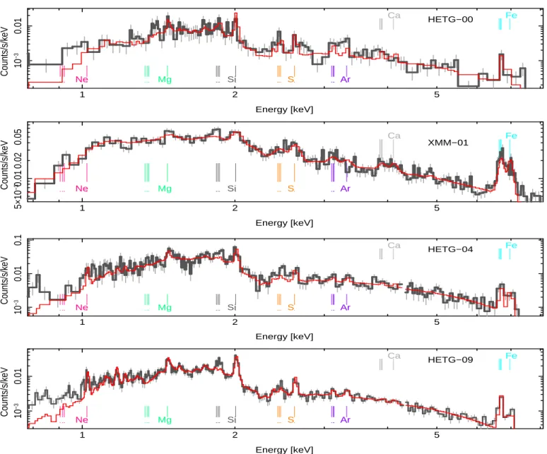
(11) Hydrodynamics and X-Ray Emission from SN 1996cr to 9.6 ×1021 cm−2 and 7.8 ×1021 cm−2 , respectively, up to 6×1021 cm−2 of which is likely from absorption in the Milky Way and Circinus Galaxy disks. We then interpolate to other epochs based on the amount of unshocked CSM. For the swept-up shell clumping, which likely extends over a range of values, we have chosen a density factor of 7.0 and a filling fraction of 0.0020; these are sufficient to generate the Si He-like lines seen at early times. The output of our calculations provides the emitted Xray flux versus time in the 0.5-2 keV band and the 2-8 keV band that we have used, as well as spectra and spectral model parameter files at each epoch. Furthermore, we have performed a detailed comparison of the line-shapes between the data and model Si and Fe lines at the HETG-09 epoch, which are described in the companion paper by Bauer et al. (2010). Figure 5 shows the comparison between the flux calculated from our hydrodynamic simulations and the observations. The abundance list used to generate these plots is given in Table 1. The separate contribution of the shocked ejecta and the shocked CSM to the flux are also shown. The modelled flux is within 20% except for the year 2000 data where it is low by 30-50 %. As Figure 3 (panel 3, 5.02 years) shows, at this time the flux is determined by the inner-half of the dense shell. We have verified (Figure 5) that shifting 10% of the dense shell mass from the outer half to the inner half can produce the needed flux increase with little change at later times. While it is tempting to expand the shape of the dense shell into a set of basis functions and adjust them for the best light curve we feel this would be “over tuning” our simple model and limited data. Certainly in future when IXO will obtain a deep, well-sampled dataset of a similar SN, such an approach could be very fruitful. It is clear that for about the first 7 years the shocked CSM material dominates the X-ray lines and the continuum, but after that the contribution of the ejecta increases as the forward shock exits the shell. By about 8 years the shocked ejecta becomes the primary contributor. If our approximation of a wind medium exterior to the dense shell is correct, then the shocked ejecta will remain the primary contributor to the total flux for more than 25 years. It is interesting to note that this is exactly the opposite scenario as deduced for another SN with a high X-ray flux, SN 1993J (Nymark et al. 2009; Chandra et al. 2009), where the reverse-shocked ejecta was found to dominate the X-ray emission for the first several decades. The dominant early contribution of the CSM is clearly due to the presence of the bubble and dense shell in this case. Our method enables us to compute simulated spectra using non-equilibrium ionization, which we can compare to the observations. Observed Chandra HETG spectra are available for 2000, 2004, and 2009, and observed XMM spectra for 2001. One important point of our method is that the same hydrodynamical simulation can produce spectra that match the observed ones at 4 different epochs, without any unnecessary free parameters. Given the transition from CSM to ejecta dominance in the emission, the CSM higher-Z abundances were obtained by using fits to both the HETG 2000 and XMM 2001 spectra, while the ejecta abundances were set by fitting to our 2009 spectrum. Figure 6 shows the comparison of the simulated and observed spectra at all the 4 epochs at which observed spectra. 11. are available. Our simulated spectra are able to fit the continuum emission very well, as well as most of the major lines (H and He-like transitions of the various lines are shown on the plot to aid the reader). We also manage to fit the line transitions in the hard X-ray band adequately. Initially, our simulated spectra did not adequately reproduce the He-like transitions of many elements, especially those that occur in the soft X-ray band below 2 keV. In order to fit these better, we assumed that there existed a component, about 1% by mass, with a density that was about an order of magnitude higher than that of the surrounding medium, and whose temperature was consequently an order of magnitude lower in order to preserve pressure equilibrium. High-density clumps may be responsible for this component. The rich and complicated line structure, at both the X-ray and optical wavelengths, is a good indicator of clumping, and the small percentage required to fit the various lines is well within the realm of possibility.. 5. SN1996CR AS A TYPE IIN - CLUMPS AND NARROW-LINE FORMATION. SN 1996cr was classified as a Type IIn supernova, based on the presence of narrow lines in the VLT spectrum from 2006 (Bauer et al. 2008). In the model presented herein, by 2006 the shock had exited the shell and was expanding in the external wind region. Thus the narrow optical lines could not arise due to the shock within the shell, whose maximum velocity in any case was much higher than the ∼ 670 km s−1 FWHM of the narrow component (Bauer et al. 2008). It is possible that the actual FWHM could be even smaller and the lines even narrower, beyond the limit of resolution of that particular observation. Could the narrow lines arise from recombination in the unshocked, ionized CSM, which we suggest (below) is a RSG wind? The velocity of the putative RSG wind would be low, . 50 km s−1 , and this line would not be resolved. In order to get the observed flux in the narrow lines, the RSG wind must have a certain minimum mass. Using equation 11 in Salamanca et al. (1998), we find that in order to get the required Hβ luminosity, a H number density in excess of 108 cm−3 is required at the position of the shock, at the time the VLT spectrum was taken (Jan 2006). This is more than 3 orders of magnitude higher than the density in our simulations, suggesting that in our scenario this line could not have come from the unshocked CSM. It is possible that the lines arise from shocked dense clumps suggested in §4.4. In order to see if this explanation is feasible, and to estimate the density, number and filling fraction of clumps, we follow the method outlined by Chugai & Danziger (1994). From the simulations, the average pressure in the shocked region at 10.5 years is about 3.9 ×10−3 dynes cm−2 . If the shock transmitted into the clump has a maximum velocity vc of 670 km s−1 (the approximate velocity of the narrow Hα line; Bauer et al. 2008) and is in pressure equilibrium, then the clump density ρc is 8.69 ×10−19 g cm−3 . Using the average value of the mean molecular weight for the CSM (see Table 1), this would mean a number density nc ∼ 6.9 × 105 cm−3 . This density is consistent with the “clumps” assumed in the previous section. The cooling time of the shock in the clumps must.

(12) 12. Dwarkadas et al.. 00. Year. 05. 10. 2-8 keV 0.5-2 keV. 1039 LX (erg s-1). FX (erg cm-2 s-1). 10-12. 10-13. 1038. 10-14 1037 1000 Days After Explosion (t - t0) Figure 5. The X-ray flux in the soft (0.5-2 keV; blue lines) and hard (2-8 keV; red lines) bands computed from our simulations, and compared to the observations (circles - error bars are shown). The data are as observed, not corrected for NH absorption. The emission from the higher density “clumps” is included, although it does not make a significant contribution to the light curve, especially at late times. An explosion date of 1995.4 is used. The individual contributions of the shocked ejecta (dotted lines) and shocked CSM (colored dashed lines) to the hard and soft fluxes is also shown. The CSM dominates the early evolution up to about 7 years, then the shocked ejecta begin to take over and dominate the later evolution. The abundances used for the figure are given in Table 1. The long-dashed grey lines indicate the light curve that would be obtained if the density profile depicted by the thin solid line in Figure 2 was used, showing how a slight rearrangement of the mass in the shell can affect the early-time light curve.. be small compared to the destruction time for the clumps by Rayleigh-Taylor and Kelvin-Helmholtz instabilities. The temperature of the shock driven into the clumps, following Chugai & Danziger (1994), is Tc = 1.36 × 107 vc28 ∼ 6.1 × 106 K. The cooling function at that temperature, from Chevalier & Fransson (1994), has a value of 5.26 ×10−23 ergs cm3 s−1 . Assuming that the cooling time is less than the time-scale on which the instabilities develop (∼ ac /vc ) gives a minimum size for the clumps of ac ∼ 1.55 × 1015 cm. As suggested by Chugai & Danziger (1994), the narrow component arises in the cool material behind the clump shock, which radiates due to the reprocessing of X-ray emission from the hot shocked gas. As the shock cools, it will progressively radiate X-ray, then UV and then optical emission from the cooling region behind the cloud shock. An upper limit to the luminosity of the ensemble of Nc shocked clumps is given by: LHα = 0.25 π a2c ρc vc3 Nc. (7). The luminosity of the narrow component of Hα is 2.79 ×1038 ergs s−1 . Using the values of ρc and vc above gives Nc ∼ 1359 ac −2 15. (8) 15. where ac15 is the clump size in units of 10 cm. Keeping in mind the lower limit on ac , we adopt ac ∼ 1016 cm, which gives Nc ∼ 13.6. The total mass in clumps is about. 0.025 M⊙ . Note that the (3D) filling fraction of the clumps, fc ∼ 1.2 × 10−3 , is quite low, and consistent with that obtained from the X-rays given the large uncertainties. The (2D) covering factor ∼ 0.027, thus indicating that they will not obscure the SN. However these clumps could add additional column density along certain sightlines. A consistency check on the above calculations can be done by comparing the ratio of the velocities. Since the clumps are in pressure equilibrium with the interclump medium, the ratio of the interclump to clump shock velocity must be proportional to the square-root of the clump to interclump density. The density of the unshocked gas at this epoch in the simulation is 1.34 ×10−20 g cm−3 . Given the density of the clumps mentioned above, the jump in density between the clumped and interclump medium is a factor of 65. If these are in pressure equilibrium, then the velocity ratios must be equal to the square-root of this, or about 8.06. Therefore, if the velocity of the shock within the clumps is 670 km s−1 , this implies that the shock velocity must be about 5400 km s−1 . This is close to the velocity of the CSM shock in our simulations (see figure 4), as would be expected. However, this is not the velocity of the broad Hα line mentioned in Bauer et al. (2008), which would be assumed to reflect the shock velocity. The inference is that either the broad Hα velocity has been underestimated, or that it does not arise from the shocked CSM, but perhaps.

(13) Counts/s/keV 10−3 0.01. Hydrodynamics and X-Ray Emission from SN 1996cr Ca. Ne. Mg. 1. Si. S. HETG−00. 13 Fe. Ar. 2. 5. Counts/s/keV 5×10−30.01 0.02 0.05. Energy [keV] Ca. Ne. Mg. 1. Si. S. XMM−01. Fe. Ar. 2. 5. Counts/s/keV 10−3 0.01. 0.1. Energy [keV] Ca. Ne. Mg. 1. Si. S. HETG−04. Fe. Ar. 2. 5 Energy [keV]. Counts/s/keV 10−3 0.01. Ca. Ne 1. Mg. Si. S. HETG−09. Fe. Ar. 2. 5 Energy [keV]. Figure 6. Comparison of the observed (black) and calculated (red) spectra at various epochs. H and He-like transitions of various elements are marked on the plot. Our simulated spectra are able to match the continuum beautifully, and the comparison with various lines is adequate. A single normalization factor is adjusted at each epoch - the spectra do not contain any other free parameters. Further details of how the spectra were calculated are given in §4.. from the shocked ejecta. Computing the FWHM of Hα depends on fitting the continuum precisely, which depends on the degree and nature of the reddening towards the SN, which is not accurately known. It is possible that the Hα has been underestimated, and that a more accurate fit to the Hα line will yield a FWHM compatible with this value. The computed values for the number, size and density of clumps are comparable to those found by Chugai & Danziger (1994), and are consistent with the “clumps” referred to in the previous section. The notion that the narrow optical lines arise in dense shocked CSM clumps, which is the same population that is also responsible for the lower-temperature (clumped) X-ray lines, is quite appealing. However the Hα lines are formed at the systemic velocity, while the X-ray lines are generally shifted by 3000-5000 km s−1 from the systemic velocity. Therefore, it appears that two separate populations may be needed.. This will be investigated further in the companion paper by Bauer et al. (2010).. 6 6.1. DISCUSSION Implications for the SN progenitor. What does our model suggest for the hydrodynamic evolution of the progenitor star? The derived density profile, with a low-density interior surrounded by a dense shell, and a wind region exterior to it, resembles a wind-blown bubble (Weaver et al. 1977) formed by the interaction of two winds. The formation of wind-bubbles, and the evolution of a SN within such wind-bubbles, has been extensively studied in the past (Ciotti & D’Ercole 1989; Chevalier & Liang 1989; Tenorio-Tagle et al. 1990, 1991; Franco et al. 1991;.

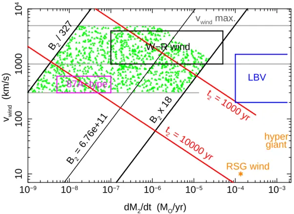
(14) 14. Dwarkadas et al.. Dwarkadas 2005, 2007a,b). These calculations have suggested that the interaction of the SN shock wave with the dense shell delineating the boundary of the wind bubble leads to increasing X-ray and radio emission. This is evidently the scenario that best resembles the emission from SN 1996cr. This is only the second case after SN 1987A where a sustained increase in the X-ray and radio light curves over a multi-year period is seen. However, the shell in the case of SN 1996cr is 6 times closer to the star than the dense equatorial ring surrounding SN 1987A. Its density in our model is a few times higher than the ring density deduced for SN 1987A. The most recent data suggest that the shock has exited the shell and the emission is turning over. Thus SN 1996cr provides an early glimpse into what the further evolution of the lightcurves in SN 1987A will look like, as the SN shock in that case is just beginning to interact with the dense equatorial ring of material (Racusin et al. 2009). In this picture, SN 1996cr represents a highly compressed, and much brighter version of SN 1987A. If we assume that the dense shell consists only of sweptup wind material, then the mass of the shell is equal to the mass of swept-up wind material. We can apply the wind bubble scenario to this model. In this scenario a fast supersonic wind sweeps up the wind from an earlier phase into a thin, dense shell. We denote the earlier phase by subscript 1 and the later phase by subscript 2. The mass of the sweptup shell is about 0.64 M⊙ . If this is made up of swept-up wind material, then Mshell = (Ṁ 1 /v1 )Rshell . Given that the shell outer radius is 1.5 ×1017 cm, this gives for the external wind a value of B1 = Ṁ 1 /v1 = 8.5e15 g cm−1 . If we assume that the wind velocity v1 is 10 km s−1 , as is appropriate for a red supergiant wind, then the mass-loss rate of the star in this phase would be Ṁ 1 ∼ 1.33 × 10−4 M⊙ yr−1 , which is again reasonable for a RSG wind. Thus one possibility is that the star in this phase may have been a RSG. If we assume a larger wind velocity, then the mass-loss rate must scale accordingly. Mass-loss rates on the order of 10−3 M⊙ yr−1 have been deduced for hypergiant stars with a wind velocity of about 40 km s−1 (Humphreys et al. 1997), and it is possible that the star in this phase could have been a hypergiant, consistent with the possibility that the progenitor was a very massive star. Even higher velocities would make it unreasonably large for any phase except perhaps the outburst stage of a Luminous Blue Variable (LBV) phase (Humphreys & Davidson 1994). But such large massloss rates are unsustainable for a large period of time, and we would expect such a phase to be necessarily short-lived (Humphreys & Davidson 1994). S Doradus type instabilities generally have a timescale of years to decades (van Genderen 2001). Therefore the existence of an LBV phase would be apparent if the density profile were to change rapidly as the shock expanded outwards, which would show up as a strong deviation in the X-ray light curve from that suggested by us in this paper. We look forward to such measurements in future. What about the final phase of the wind before the star exploded? Only upper limits to the X-ray emission are available for this period, thus only providing an upper limit to the density profile. In the simulations, we assume a wind with a value of B2 = Ṁ /vw = 6.76 ×1011 g cm−1 , which we refer to as the standard value of B2 . This means that for a wind velocity of a 1000 km s−1 , the mass-loss rate is on. the order of 10−6 M⊙ yr−1 (Figure 7). The wind density is most constrained by the upper limits on the X-ray emission between days 600-900. A factor of 18 increase in the value of B2 delays the high-flux turn-on and increases the discrepancy for the year 2000 measurements by 20 to 30 % . Thus the maximum mass-loss rate that would be able to produce a reasonable light curve (within 30% of the observed values) and just about satisfy other constraints (for a velocity of 1000 km s−1 ) would be about 1.8 ×10−5 M⊙ yr−1 . At the lower end we find that the density could be significantly smaller before the shock collides with the dense shell too early and exceeds the upper limits on days 700900 (although this can be somewhat mitigated by changing the explosion date, which is uncertain by about a year). For the same 1000 km s−1 velocity, we find a lower-limit to the mass-loss rate of about 3.26 ×10−9 M⊙ yr−1 . Thus, although we cannot exactly constrain the inner density, we find that the best fit light curve leads to mass-loss rates between 3. ×10−9 M⊙ yr−1 and 2. ×10−5 M⊙ yr−1 , for wind velocities of 1000 km s−1 . At the higher end, this mass-loss rate would be compatible with a Wolf-Rayet star progenitor for the SN. This would make the SN a Type Ib/c. At the lower end, and especially for lower velocities, the mass-loss rate and wind velocity combination approaches that deduced for SN 1987A (Chevalier & Dwarkadas 1995; Lundqvist 1999; Dwarkadas 2007c,b), and may further strengthen the analogy between SN 1996cr and SN 1987A. While we are not suggesting that the progenitor of SN 1996cr was a blue supergiant, it lies within the realm of possibility. One implication of these low mass-loss rates is that it is unlikely that the progenitor star was an LBV star. LBVs are highly luminous, unstable stars, which can undergo episodes of dramatic mass-loss (Humphreys & Davidson 1994), leading to the formation of circumstellar nebulae around the star. LBV nebulae are generally of order 1pc (Weis 2001), much larger than the circumstellar nebula in our simulations. LBV stars have often been suggested as progenitors for Type IIn SNe (Gal-Yam et al. 2007; Smith 2008; Vink 2008; Gal-Yam & Leonard 2009; Miller et al. 2009), based mainly on the fact that they undergo mass-loss episodes with a high mass-loss rate & 10−4 M⊙ yr−1 . LBV winds are also slower than W-R winds, with velocities on the order of 200 km s−1 (Vink & Kotak 2007). Assuming such a velocity would lower the mass-loss rates derived above by a further factor of 5. This would lead to mass-loss rates lying between about 6 ×10−10 M⊙ yr−1 and 4 ×10−6 M⊙ yr−1 (see Figure 7) for a presumed LBV progenitor velocity. These are significantly lower than mass-loss rates proposed for LBV progenitor stars. Mass-loss from an LBV in the quiescent stage may be consistent with the higher end of the rates deduced here (Humphreys & Davidson 1994), but then it is impossible to distinguish this from other massive supergiant stars (Stothers & Chin 1996) based purely on hydrodynamic considerations. In any case by assumption this would indicate that the wind bubble was not the result of an LBV outburst. We can further constrain the wind parameters by including the shell formation time, t2 . As above, we assume that the shell was formed by the interaction of two winds with constant mass-loss parameters, the first wind being the earlier RSG wind, followed by the second wind phase. The shell radius is given by Rshell = (L2 /[1.5B1 ])1/3 t2 cm.