TítuloTopological active model optimization by means of evolutionary methods for image segmentation

(1)

Facultade de Inform´

atica

Departamento de Computaci´

on

PhD Thesis

Topological Active Model Optimization

by Means of Evolutionary Methods for

Image Segmentation

Author: Jorge Novo Buj´an

(2)

(3)

To my mother Mar´ıa and brothers Manuel, Ram´on, Lu´ıs and Julio. And especially, in memory of my father Ram´on.

(4)

(5)

Acknowledgements

I would like to mention, in the first place, my supervisors Jos´e Santos Reyes and Manuel Francisco Gonz´alez Penedo for letting me have the opportunity to do this PhD thesis. Thanks for all the help, suggestions and supervision during these years that have made this work possible.

I especially thank my colleagues Marcos, Noelia, Jos´e, Vero, Cas, Marta, Bea and the rest of the members of the VARPA group for all the support, collaborations and shared moments during all this time.

I would also like to express my gratitude to my family and friends. My mother and brothers, thanks for supporting me when I took this path in my career and for being there any time I needed. My godson, my nephew, the rest of my family, my friends of Bandeira and A Coru˜na, you were always there making everything easier. Finally, I would like to dedicate this work in memory of my father. You worked so hard all your life to give us the chance to make our dreams come true, but, unfortunately, you cannot be here to enjoy this moment with us. I hope you were proud up there.

(6)

(7)

Preface

Object localization and segmentation are tasks that have been growing in relevance in the last years. The automatic detection and extraction of possible objects of interest is a important step for a higher level reasoning, like the detection of tumors or other pathologies in medical imaging or the detection of the region of interest in fingerprints or faces for biometrics.

There are many different ways of facing this problem in the literature, but in this Phd thesis we selected a particular deformable model called Topological Active Model. This model was especially designed for 2D and 3D image segmentation. It integrates features of region-based and boundary-based segmentation methods in order to perform a correct segmentation and, this way, fit the contours of the objects and model their inner topology. The main problem is the optimization of the structure to obtain the best possible segmentation. Previous works proposed a greedy local search method that presented different drawbacks, especially with noisy images, situation quite often in image segmentation.

This Phd thesis proposes optimization approaches based on global search meth-ods like evolutionary algorithms, with the aim of overcoming the main drawbacks of the previous local search method, especially with noisy images or rough contours. Moreover, hybrid approaches between the evolutionary methods and the greedy local search were developed to integrate the advantages of both approaches. Additionally, the hybrid combination allows the possibility of topological changes in the segmen-tation model, providing flexibility to the mesh to perform better adjustments in complex surfaces or also to detect several objects in the scene.

The suitability and accuracy of the proposed model and segmentation methodolo-gies were tested in both synthetic and real images with different levels of complexity. Finally, the proposed evolutionary approaches were applied to a specific task in a real domain: The localization and extraction of the optic disc in retinal images.

(8)

(9)

List of Figures

1.1 Examples of medical images . . . 1

2.1 A 6×6 TAN mesh . . . 14

2.2 A 4×4×3 TAV mesh . . . 19

2.3 3D link cutting example . . . 23

2.4 3D multiple breaking example . . . 24

2.5 Threads and cutting priorities in 2D . . . 25

2.6 Threads and cutting priorities in 3D . . . 25

2.7 Segmentation process using a greedy strategy diagram . . . 26

2.8 Wrong segmentations using the greedy methodology . . . 27

3.1 Standard genetic algorithm process . . . 32

3.2 Arithmetical crossover operator . . . 35

3.3 Mutation operator . . . 36

3.4 Spread operator . . . 37

3.5 Group mutation operator . . . 38

3.6 Shift operator . . . 38

3.7 Results at the end of each phase using a GA process . . . 41

3.8 GA method. Results obtained in an image with fuzzy contours . . . 43

3.9 GA method. Results obtained in an image with Gaussian noise . . . 44

3.10 GA method. Results obtained with irregular noise . . . 44

3.11 Hybridized GA method. Example of segmentation with a breaking sequence . . . 47

3.12 Hybridized GA method. Example of segmentation with several ob-jects in the scene . . . 48

3.13 Hybridized GA method. Results obtained in an image with fuzzy contours . . . 50

3.14 Hybridized GA method. Results obtained in an image with Gaussian noise . . . 50

(14)

xii LIST OF FIGURES

3.15 Hybridized GA method. Results obtained with irregular noise . . . . 51 3.16 Hybridized GA method. CT image segmentation that requires

topo-logical changes . . . 51 3.17 Hybridized GA method. CT image segmentation that requires the

division of the mesh . . . 53 4.1 Example of 2D calculation of a candidate solution (Xcandidate) to

re-place a given individualX using DE . . . 56 4.2 Comparison of GA and DE methodologies in 2D . . . 61 4.3 Best individual fitness and average fitness of the population with the

GA and DE processes in 2D . . . 62 4.4 Best individual fitness and average fitness of the population with the

GA and DE processes in 3D . . . 63 4.5 Best individual across generations in GA and DE processes in 3D . . 64 4.6 Best individual evolution comparing the DE approach with different

hybrid approaches and the greedy method in 2D . . . 66 4.7 Best individual evolution comparing the DE approach with different

hybrid approaches and the greedy method in the 3D case . . . 67 4.8 Best final results obtained using the hybridized DE in noisy 2D images 68 4.9 Final result obtained using the hybridized DE in a CT noisy 3D image 68 4.10 2D image segmentations that require topological changes using the

hybridized DE . . . 69 4.11 3D image segmentations that require topological changes using the

hybridized DE . . . 70 4.12 2D image segmentations that require division of the mesh using the

hybridized DE . . . 71 4.13 3D image segmentations that require division of the mesh using the

hybridized DE . . . 72

5.1 Example of Pareto Set using 2 objectives . . . 77 5.2 Example of the neighborhood considered for the calculation of the

k-distance of the central node . . . 82 5.3 Hybridized SPEA2-GA results obtained in the segmentation of a circle 84 5.4 Representation of the Pareto Front in a segmentation process using

the hybridized SPEA2-GA . . . 87 5.5 GA and hybridized SPEA2-GA results in the segmentation of different

(15)

LIST OF FIGURES xiii

5.6 GA and hybridized SPEA2-GA results in the segmentation of artificial images . . . 91 5.7 GA and hybridized SPEA2-GA results obtained in the segmentation

of complex objects . . . 92 5.8 GA and hybridized SPEA2-GA results in the segmentation of complex

objects . . . 93 5.9 GA and hybridized SPEA2-GA results in segmentations with CT images 94 5.10 Hybridized SPEA2-GA results obtained in the segmentation with real

images . . . 95 5.11 Best value of the IODi/GD objective of the population with the

different MO processes in 2D, using SPEA2-GA and SPEA2-DE hy-bridizations . . . 98 5.12 2D sequence of the best individual (accordingIODi/GDobjective) in

different generations using SPEA2-GA and SPEA2-DE hybridizations 99 5.13 Best value of the IODi/GD objective of the population with the

different MO processes in 3D, using SPEA2-GA and SPEA2-DE hy-bridizations . . . 99 5.14 3D sequence of the best individual of the Pareto Set according the

IODi/GDobjective, using SPEA2-GA and SPEA2-DE hybridizations 100

5.15 Results of the comparison between the hybridized SPEA2-DE and single-objective DE using a CT image of the knee . . . 101 5.16 Hybridized SPEA2-DE results obtained in the segmentation of 2D

examples . . . 103 5.17 Hybridized SPEA2-DE results obtained in the segmentation of 3D

examples . . . 103 5.18 Hybridized SPEA2-DE results obtained in the segmentation of the

humerus in medical CT images . . . 104 6.1 Example of retinal image focused on the macula, including the main

characteristic structures . . . 108 6.2 Optic disc segmentation. Example using the contrast of intensities . 113 6.3 Optic disc segmentation. The two initialization processes . . . 114 6.4 Optic disc segmentation. Example of GA evolution without the

cir-cular structure energy term . . . 117 6.5 Optic disc segmentation. Example of GA evolution without the

en-ergy term of the intensity contrast . . . 119 6.6 Optic disc segmentation. Final result obtained with the greedy

(16)

xiv LIST OF FIGURES

6.7 Optic disc segmentation. Segmentation results, used for localization, on images with the optic disc in the center . . . 122 6.8 Optic disc segmentation. Results using different TAN resolutions . . 123 6.9 Optic disc segmentation. Segmentation results, used for localization,

over images centered on the macula . . . 124 6.10 Optic disc segmentation. Localization examples in images with

exu-dates and other bright areas . . . 125 6.11 Optic disc segmentation. Analysis of differences among

ophthalmol-ogist localizations and results of the method . . . 126 6.12 Optic disc segmentation. Two localization examples with difficult

images from the VARIA database . . . 127 6.13 Optic disc segmentation. Analysis of differences among

ophthalmol-ogist localizations and results of the method . . . 128 6.14 Optic disc segmentation. Hybridized SPEA2-GA results in the

seg-mentation of a typical retinal image . . . 129 6.15 Optic disc segmentation. Hybridized SPEA2-GA results obtained in

the segmentation with the incorporation of the ad-hoc energy terms as objectives . . . 130 6.16 Optic disc segmentation. Hybridized SPEA2-GA results obtained in

the segmentation of a retinal image that presents pathologies . . . . 132 6.17 Optic disc segmentation. Hybridized SPEA2-DE results obtained in

(17)

List of Tables

3.1 TAV parameter sets of the 1st evolutionary phase in the segmentation processes of the examples using GA approaches . . . 42 3.2 TAV parameter sets of the 2nd evolutionary phase in the segmentation

processes of the examples using GA approaches . . . 42 3.3 GA parameters used in the evolutionary processes using GA approaches 43 3.4 Comparison between the greedy local search and the GA approaches 53 4.1 TAN and TAV parameter sets used for the segmentation of the image

examples using DE approaches . . . 60 4.2 Comparison between the GA and DE approaches . . . 73 5.1 TAM parameter set of the GA first phase in the segmentation

pro-cesses of the examples, in the comparisons with the SPEA2 approach 86 5.2 TAM parameter sets of the GA second phase in the segmentation

processes of the examples, in the comparisons with the SPEA2 approach 86 5.3 Genetic operators probabilities used in the GA and SPEA2 processes 86 5.4 TAN parameter set used for the segmentation of the image of Figure

5.15, using DE . . . 100 5.5 Comparison between the single-objective methods (GA and DE) and

the SPEA2 approaches . . . 105 6.1 TAN parameter sets in the optic disc segmentation processes . . . . 118 7.1 Comparison among the different optimization methods . . . 137

(18)

(19)

Chapter 1

Introduction

In the recent years, the automatic processing of 2D and 3D image datasets became a relevant task in the way the datasets to be processed and analyzed were extremely increased in many professional areas. For example, in the medical domain, novelty technologies such as Computed Tomography (CT), Magnetic Resonance Imaging (MRI), or more specifically in ophthalmology, Optic Coherence Tomography (OCT) or retinal images, provide new information and points of view of real structures of the patient. All this information has to be processed and analyzed by the specialists for medical treatment. Figure 1.1 shows some examples of the different medical images mentioned.

Despite the fact that it is a relatively recent area, the digital image processing has demonstrated its great usefulness in the automatic treatment of image datasets. Some of the tasks involved can be, for instance, the morphological image processing, the image recognition or the interpretation systems. Thus, digital image processing can help the specialists to process large datasets, replacing manual procedures which

(a) (b) (c) (d)

Figure 1.1: Examples of medical images. (a) CT slice. (b) MRI scan: a short axis mid ventricular cardiac magnetic resonance for heart analysis. (c) OCT image. (d) Retinal image.

(20)

2 1. Introduction

require long time.

The relevance acquired by the different methods of digital image processing is due to two main areas of application:

Improvement in the image characteristics for human comprehension The aim is the improvement of the quality of the image to be analyzed by a spe-cialist. This kind of techniques are used in different areas, like communication systems or military intelligence.

Processing of the data in a scene The aim is the autonomous interpretation by the machine. That is, the machine can understand what is processing as input information, and to extract the relevant information in the images of interest that corresponds with a real scene and give it a meaning.

Therefore, for this second issue, computer vision techniques can be applied in order to extract and analyze the features of interest in the scene. This issue needs a procedure of different levels of complexity. This implies:

• Detection and segmentation of the objects or regions of interest in the scene. • Extraction of the characteristics or topological and morphological parameters

of these objects or regions.

• Identification and classification of the objects or regions.

• Image understanding of the scene once the objects or regions have been iden-tified.

In this sense, image segmentation and object extraction are crucial tasks in the image understanding process in several domains. One of the most important is medical imaging, where the image understanding is a relevant issue for different tasks: computer-aided diagnosis, surgery planning and simulation or radiotherapy planning, among others. However, these processes normally are complicated because the images are not as ideal as desired. Most of the times, the machines capture the images of interest not perfectly, acquiring the data with different artifacts or noise, making the understanding process more difficult. For that reason, as a crucial task, the segmentation process needs to be as robust as possible, under any possible circumstance.

(21)

1.1. Image segmentation 3

and we applied different evolutionary methods for its optimization. This chapter details a general review about the different issues related with such tasks, beginning with an explanation about image segmentation, following with the main principles and works related with deformable models and ending, more specifically, with the related work in the literature that used evolutionary computation to deformable models.

1.1 Image segmentation

As we described before, one of the first steps in the process of image understanding consists of segmenting the image of interest. This segmentation subdivides the image in different parts or regions that constitute the entire scene. The level of subdivision depends on the desired characteristics to be analyzed.

The efficiency of the segmentation is crucial for a process of image understanding, because it is the task responsible of extracting the regions of interest. Due to the data size and the possible variability of the features, the different levels of noise in the images, sampling artifacts or spatial aliasing that can sometimes cause blurred or disconnected boundaries, under all these possible situations the segmentation can be a challenging problem. For that reason, as we explained before, the segmentation technique has to be as much robust as possible to extract the desired objects or regions as better as possible, depending on that the success of any computer vision technique.

The principles of segmentation have their origin in the psychological works of the Gestalt [59], that studied the preferences of the human beings in the organi-zation of groups of shapes in the vision field. These principles indicated that the human being has some specific preferences in the way they organize the perception, based on certain characteristics like proximity (objects near among them tend to be grouped together), similarity (objects that are similar among them tend to be grouped together) and continuity (objects that conform a close entity tend to be grouped together). This is the way the perception of the human being works. How-ever, these principles are highly difficult to implement in a machine process and different authors in the literature had to develop many different approximations to perform the segmentation.

(22)

4 1. Introduction

[38]:

Segmentation based on regions The main idea consists of dividing the entire image in different regions, grouping the pixels that belong to one object to-gether. The criteria to group the different points is normally a similarity measure based on properties of a given point and its neighborhood. Examples are clustering methods or region-growing methods.

One of the most used methodologies regarding this category are the graph cuts methods [15]. The main idea consists of formulating the segmentation problem as a energy minimization. Representing our problem as a graph, the energy minimization problem can be reduced to instances of the maximum flow problem in the given graph, defining the minimal cut of the graph as well (as detailed by the max-flow min-cut theorem [75]), that represents the best contour of the object to be segmented. There are different versions based on graph cuts, becoming very famous segmentation methods.

Segmentation based on contours or edges They are normally based on the principle that a change in intensity (an edge) points out the separation of two different objects. Thus, the detection of different objects or regions uses the information of edges in the image of interest. An example of this kind of methods are edge detectors. One of the most famous techniques under this category are thelevel sets method. It is explained later in Subsection 1.2.2. There are different organizations based on different characteristics. Additionally to the previous categorization, one of the simplest and most used classifications is based on the complexity of the method, having that way low-level and high-level techniques [104, 76]. The main principles are:

Low-level techniques These methods are based on simple characteristics of the image, like levels of intensity or the extraction or edges. The simplest are the thresholding methods. They basically turn a grey-scale image into a binary one using a threshold value. There are other methods in this category like histogram based methods or classifiers. The main characteristics of these methods are their simplicity and the efficiency, but they have many problems in the achievement of accurate results in complex images, like noisy images, objects with fuzzy contours or discontinuities, etc.

(23)

1.2. Deformable models 5

they normally extract a model related with the objects or regions of interest. As they integrate different features to perform the localization and segmentation, these methods are more robust to the possible complications in the segmentation process and normally obtain better results than the low-level techniques. They also provide structural information of the objects of interest. However, these methods are pe-nalized in efficiency, normally having higher complexities than the low-level ones. Under this category we can find segmentation techniques like deformable models [51], Bayesian methods [79] or atlas-guided techniques [4]. These methods are nor-mally more suitable for image segmentation because they provide better results in complex domains and also provide topological and morphological information about the segmentations achieved.

Regarding image segmentation, one of the most used paradigms is deformable models, where is enclosed the proposed work is enclosed. In the next section, we will explain the main basis and related work about the deformable models field.

1.2 Deformable models

One of the most used high-level technique is deformable models. Given the limi-tations of the low-level techniques, Kass et al. proposed a deformable contour in 2D [51] that was also extended to 3D by Terzopouloset al. [97], providing a global solution to the segmentation problem based on the localization of contours. This new way of approaching the image segmentation task implied an improvement with respect to the classic approaches previously defined. Thus, deformable models pre-sented a better way of dealing with the difficult task of segmentation in images with noise or sampling artifacts, or the presence of objects with fuzzy or discontinuous contours. In addition to that, the aim of the segmentation process is not only the extraction of the points that belong to a given object or region, but also to extract its relevant characteristics. Thus, deformable models extract the boundary of the objects and also provide their main features, reconstructing a representation of the structure.

They have been used for several different tasks, like pattern recognition [2, 30], computer animation [95], geometric modelling [47], surgery simulation [29], tracking [13] or image segmentation [50, 67, 108], among others. One of the specific domains where they were widely used is the medical image analysis. Some surveys detail the work related in this field [63, 85].

(24)

6 1. Introduction

the given domain by a set of forces, both internals and externals. These forces can be described from two different points of view. In a physical point of view, the characteristics of the image determine the external forces, meanwhile the internal forces control the smoothness of the model during the deformations. Moreover, from a mathematical point of view, a deformable model is moved under its dynamic equations, trying to minimize an energy function associated to the model. This energy function represents the correctness of the adjustment, that is, the better the model fits the objects, the lower is the energy.

There is an entire world of deformable models based on different characteristics. In the survey of Montagnatet al. [68] the authors explain the main ideas of several deformable models developed. According to their classification, we can organize all the variety of deformable models regarding some relevant characteristics.

1.2.1 Features used as the energy function

As we indicated, the deformable models are deformed according to a set of forces. These forces are represented by different characteristics like image features -for ex-ample image intensity or proximity to edges- and model features -like smoothness and contraction-. Most of the deformable models use these forces as a summed en-ergy term that represents the correctness of the adjustment to the objects, that is called the energy function.

One of the first models in the literature was the snake [51]. This model is a parametrized model that evolves according to the minimization of an energy func-tion. This energy function includes internal forces, controlling the smoothness and rigidity of the structure, and also external forces, represented by the image features that attract the model to the contour of interest. This approach is simple but robust against noise and missing data. Nevertheless, it is highly dependent on the contour parametrization and the initialization of the model in the image.

After this first approximation, other different models were developed, including different characteristics. For instance, Cohen [24] proposed a model called balloon, that is basically an approximation of the model to a sphere by means of polygons. This model can be inflated or deflated until the contour is reaching a contour.

(25)

a new model calledgradient vector flows [105], that uses the same principles but it is based on smoothing the gradient field of an image edge map with a non–linear partial differential equation. This way, the attraction range of the image boundaries is extended to the whole image domain.

There is other way of using the image information to perform the segmentation. Thus, instead of using the boundary information, we can use region information. Chan and Vese proposed a new method called active contours without edges [19] that mainly performed the minimization of the Mumford-Shad functional [69] with a level set based technique.

Regarding the energy function in all the models, any characteristic with useful information added to the energy function is desired. Thus, if we are working in a given domain, some domain knowledge can be included in the energy function. Thanks to that, the model is more robust to complications in the images, obtaining better results. An example of this kind of models are theactive shape models[41, 26] andactive appearance models[32, 25] that use statistical information from a training set of images that contain the features of interest.

1.2.2 Deformable models geometry

One of the main characteristics remains in the fact that a deformable model can be characterized by its surface representation, according to the shape description (the model is restricted to represent simple shapes, shapes of restricted topology or shapes with different topologies) and thedeformation description (by deforming directly the shape or deforming its embedding space, for instance, applying global transformations to the model).

Continuous and discrete representations As a first differentiation regarding geometry, we can have deformable models that present continuous and discrete repre-sentations. With a continuous representation we can compute differential quantities, such as surface normals and curvatures, almost everywhere on the surface. Mean-while, with discrete ones, the surface is only known in a specific set of points. The main problem of the continuous representations is the computational requirements, needing most of the time to be discretized.

Explicit and implicit representations Basically, explicit models are repre-sented by a set of parameters or coordinates, meanwhile implicit models involve an implicit equation to locate the surface points.

(26)

8 1. Introduction

from where the B-snakes [65], which basically is a B–spline representation of a snake, and its improved version that allows topological changes [56, 55] are the most fa-mous ones. One of the most used ones are thesuperquadrics [94, 8], which basically represents closed surfaces. Such models only allow the representation of symmetric shapes discarding complex surfaces. We also have other types like deformable tem-plates, that basically use a set of allowed templates for a specific segmentation, like in the work of Yuilleet al. [109], or modal decompositions, that use a set of different frequency harmonics [86, 89].

Regarding implicit models, we can findalgebraic surfaces [92, 93],superquadrics, that, in addition to the explicit representation, they can also being formulated in an implicit way [8], orhyperquadrics, which is an extension of the superquadric models [23, 22, 39].

Nowadays, one of the most used techniques under implicit representation mod-els is the level sets method, technique that was proposed by Osher and Sethian [74] and fully described in [84]. At the first moment, it was proposed for tracking moving interfaces, but then its use spread to other imaging domains, like medi-cal applications [62]. The procedure mainly represents the deformable model as a higher-dimensional scalar function. The contour or surface of the object is the zero-level set of points, where each point is represented as the distance from this point to the higher-dimensional model. Thus, the distance is positive for all the points outside the surface and negative for those that are inside, meanwhile the contour of the segmentation is composed by the set of points with values equal to zero. The evolution of the surface is guided by a partial differential equation regarding the higher-dimensional scalar function that represents the model. The main advantage of this approach is that changes in the topology are allowed easily and implicitly to the model. On the contrary, the main drawback consists of the computational requirements, that is, the numerical solution of the level set equation requires so-phisticated techniques, representing the main challenge of the method.

1.2.3 Deformable models evolution

(27)

models in terms of reducing the associated energy function.

There are many different techniques to develop this task. One of the easiest way is using agreedy strategy like in the work of [103]. The main idea consists of modifying locally the model in a way of reducing the energy until no further modification implies a reduction in terms of energy. As an advantage, these methods are fast in reaching the results, but they are also sensitive to possible noise or complications in the images.

Considering all the complications that can be presented in the datasets, the localization of the global minimum, or at least one acceptable local minimum, is not a trivial issue. There were some approximations like theBayesian approach that uses a statistical framework to do the minimization [88, 109]. Along this line, Terzopoulos and Szeliski [96] depicted a “Kalman snake”, based on a probabilistic modelling by adding a Kalman filter to prior models and data with a Bayesian method.

Other global search techniques were developed that become popular and provide acceptable results with a minimum of guarantees. Some of the most used methods are related with the simulated annealing [87], dynamic programming [3] or graph cuts [14], that have been widely used in the literature.

The global search methods minimize the problem of falling in local minima. Among them, we used evolutionary methods as searching algorithms or minimization methods for our deformable model.

1.2.4 Evolutionary approaches and deformable models. Related work

(28)

10 1. Introduction

Tanatipanond and Covavisaruch [90, 91] also applied a GA to optimize snakes in brain MR images. They used a multiscale approach, beginning at coarser scales to extract rough contours. Then, the best deformable contours at this stage were the parent chromosomes at finer scales. S´eguier and Cladel [82] used genetic snakes in a speech recognition application that integrates information from audio and the visual processing of the mouth. In their approach, there were two snakes that define the lips contours and converge in parallel.

Tohka and Mykk¨anen [100] improved the results of deformable surface meshes by means of a dual contour method in Positron Emission Tomography (PET) brain im-ages. Tohka also used a hybrid approach in [99], where a GA globally minimized the energy of a deformable surface mesh. The minimum obtained was further strength-ened by a greedy algorithm. The GA detected roughly the target objects and then the greedy search was used for precise surface extraction.

In other works it was proved the superiority of a global search method by means of a genetic algorithm ([37]) in the optimization of the Topological Active Nets in 2D images ([45, 81]). The results showed that the GA is less sensitive to noise than the greedy algorithm and does not depend on the parameter set or the mesh size.

In the case of 3D segmentation contours, Bro-Nielsen [16] used 3D “active cubes” to segment medical images, where the automatic net division was a key issue. How-ever, they did not use GAs, only an improved greedy algorithm inspired by a simu-lated annealing procedure to overcome the noise problems.

1.3 Objectives

(29)

1.3. Objectives 11

deformable models because they allow the extraction of the surfaces and also the analysis of the features of the inner of the objects. In both approximations, the nodes are organized as a mesh that has to be deformed under the influence of differ-ent functions that conform the energy of the model. Moreover, as other advantage of these deformable models, we can perform topological changes in the model structure to provide flexibility to the mesh, and to perform better adjustments in the presence of holes, concavities or even the segmentation of several objects in the scene.

As explained for other deformable models, the Topological Active Models are governed by an energy function that weights the correctness of the segmentation developed by the model, in such a way that the lower is the energy the better is considered the segmentation performed. As we explained before, the images can present different complications (noise, artifacts captured, boundary discontinuities, etc., ...), that makes the process of segmentation (minimization of the mesh energy) a complex issue.

A previous segmentation technique [9] was developed to minimize the energy using a greedy method. As an advantage, a greedy approach is fast, but it has many problems to reach acceptable results under the detailed complications that can appear in a given dataset. For that reason, global search methods are more suitable for the problem, especially if we focus the properties of the method on the robustness. Thus, in this work, different global search methods using evolutionary approaches were developed trying to overcome the limitations of the previous technique, that is, the greedy local search. Moreover, some hybridizations using the evolutionary global search methods and the greedy local search were performed with the aim of integrate the properties and advantages of both ways of facing the adjustment of the models.

1.3.1 Organization of the thesis

This thesis describes all the evolutionary approaches developed for the image seg-mentation task, detailing the characteristics of all the methods and the results ob-tained for each of them.

Chapter 2 discusses all the characteristics of the Topological Active Models (both TAN and TAV models) regarding the topology and the composition of the energy function associated. Moreover, the chapter includes the description of the greedy local search previously developed for the adjustment of the model and also the mechanisms used to perform the changes in the topology.

(30)

12 1. Introduction

the domain and also new ad hoc genetic ones were proposed. In the chapter, the entire evolutionary process is described. Moreover, an entire set of experiments are shown to demonstrate the advantages of the global search approach with respect to the greedy local search previously defined. Different difficulties like noise or fuzzy boundaries were used in the experiments. A hybridization of both methodologies is also shown with the corresponding results.

The adapted GA approach presents several limitations. One of them is the slow convergence of the method over the desired results. Chapter 4 describes one of the improvements. A new evolutionary approach, and also the hybridization with the greedy local search, based on Differential Evolution, is used. Representative results are shown and also a comparison between the new evolutionary method and the GA approach was performed, to demonstrate the advantages of the alternative evolutionary method.

One of the important drawbacks of all the single-objective methods, including the proposed evolutionary approaches, in this particular problem, consists of tuning all the energy parameter set. The energy of the model used is defined by different components, weighted by different parameters that measure the relevance of each component in the entire energy function. This parameter tuning has to be devel-oped for each image segmentation, trying to obtain the best possible results in each situation. Chapter 5 explains all the basis of the alternative methodology based on multiobjective optimization. This technique overcomes the limitation of the pa-rameter tuning. Different results and the comparison with the GA approach are shown.

Moreover, in Chapter 6, we include a practical application in which the segmen-tation techniques developed were used: We used the methods in the task of detecting and segmenting the optic disc in retinal images. A large set of tests was developed to validate and show the robustness of the approximations.

(31)

Chapter 2

Topological Active Models

The Topological Active Net (TAN) [5] and its 3D extension, the Topological Active Volume (TAV) [9] are discrete implementations of an elastic n−dimensional mesh with interrelated nodes that integrates features of region–based and boundary–based segmentation techniques, generally called Topological Active Model (TAM).

As other deformable models, the state of the model is governed by an energy function composed by different energy terms related to the mesh nodes. This func-tion weights the correctness of the segmentafunc-tion so the adjustment process is based on its minimization.

This chapter details the mesh topology and the energy formulation in the TAN model and explains how the 2D model is extended to 3D, emphasizing on the en-ergy terms that represent the objectives to be optimized with the evolutionary ap-proaches. The chapter ends with the description of the initial strategy used for the minimization of the energy of the mesh, a greedy method which incorporates the possibility of changes in the topology of the initial mesh.

2.1 Topological Active Nets

Topological Active Nets are a 2D deformable model based on the Active Nets model proposed by Tsumiyama et al. [101] and developed by Bro-Nielsen [16]. The TAN model shares with those approaches the mesh topology as well as the base energy def-initions. However, the TAN model proposes different energy functions and performs different segmentation stages that widen the application fields of the model.

This section explains the bases of the TAN model regarding the initial mesh configuration and the related energy functions.

(32)

14 2. Topological Active Models

2.1.1 Topology

A Topological Active Net is a two–dimensional mesh formed by interrelated nodes. The model distinguishes two types of mesh nodes: internal, inside the mesh, and external, on the boundaries. Each type of node represents different features of the objects. The external nodes fit the object surfaces, whereas the internal nodes model the inner object features. This way, the segmentation process integrates boundary and region information in the segmentation process [5, 9]. Figure 2.1 shows a TAN mesh that contains both types of nodes.

Figure 2.1: A 6×6 TAN mesh. The external nodes are on the boundaries (in blue), whereas the internal nodes are inside the mesh (in green).

As figure 2.1 shows, the TAN nodes are arranged in a polygonal grid formed by squares or rectangles. The edges of these polygons define the neighboring re-lationships between nodes. Hence, the internal nodes have 4 neighbors, whereas the external ones only have 2 or 3 neighbors regarding their position on the mesh boundaries. The mesh connectivity has influence on the deformation process as well as on the segmentation results, as it will be explained later.

2.1.2 Energies

The TAN model is defined parametrically asv(r, s) = (x(r, s), y(r, s)) where (r, s)∈ ([0,1]×[0,1]). The mesh deformations are guided by the following energy function:

E(v(r, s)) =

Z 1

0

Z 1

0

Eint(v(r, s)) +Eext(v(r, s))drds (2.1)

where Eint stands for the internal energy and Eext is the energy due to external

(33)

2.1. Topological Active Nets 15

the features of the scene that guide the adjustment process.

Internal energy objectives The calculus of the internal energy term depends on first and second order derivatives:

Eint(v(r, s)) = α(|vr(r, s)|2+|vs(r, s)|2)

+ β(|vrr(r, s)|2+ 2|vrs(r, s)|2+|vss(r, s)|2)

(2.2)

where the subscripts represent the partial derivatives andα, β are weighting terms that control the contraction and bending, respectively. On one hand, large values of α increase the mesh contraction, whereas small values of α restrict the mesh contraction. On the other hand, large values of β produce smooth curves in the mesh, whereas small values ofβ allow sharp edges.

The definition of the internal energy in 2.2 is continuous. However, the image is a discrete domain. For this reason, the parameter domain [0,1]×[0,1] is discretized as a regular grid defined by the internode spacing (k, l) and the partial derivatives are computed using the finite difference technique. In this technique, the derivatives are approximated by finite difference formulae based on values of the function at discrete points.

The first order derivatives can be computed using the following approximations:

d+

whered+,do_and_d−_{are the forward, centered and backward differences, respectively.}

In the TAN case, the central difference formula cannot be used for the estima-tion because it only takes into account the contribuestima-tion of the neighboring nodes. Note that the segmentation process is an energy minimization task and the min-imization process is based on changing the position of one or several mesh nodes and comparing the energy values. If the first derivatives are computed by means of the central estimator, when a node changes its position, the first derivative term remains unchanged unless its neighboring nodes have been also updated. Therefore, the central estimator does not allow the evaluation of the quality of the new node position in these cases.

(34)

for-16 2. Topological Active Models

On the contrary, the second order derivatives are estimated using the standard finite difference technique since it takes into account the position of the current node:

vrr =

External energy objectives While the internal energy term controls the con-traction and bending of the TAN, the external energy term represents the features of the scene that guide the adjustment process. This term is defined in such a way that local minima coincide with the image features to segment.

In the TAN model, the external energy of a node is defined as a function of the image intensity and takes into account the neighborhood in the computation. This way, the external energy of a node not only depends on the node itself, but also on the information provided by its neighboring nodes in order to increase the robustness of the segmentation process and avoid local minima caused by noise or intensity inhomogeneities. Hence, the external energy term is defined as follows:

Eext(v(r, s)) =ωf[I(r, s)] +

where ω and ρ are weights, I(v(r, s)) is the intensity value of the original image in the position v(r, s), f is a function related to the image intensity, and ℵ(r, s) is the mesh neighborhood of the node (r, s). Thereby, the mesh topology has influence in the energy computation. Note that the contribution of each neighboring node is inversely proportional to its distance to the current node so that the information provided by the closest neighbors has more relevance. This fact ensures a more stable mesh deformation.

(35)

2.1. Topological Active Nets 17

should be defined in such a way that the internal nodes will remain in the interior of the objects, whereas the external nodes will be attracted by the object boundaries. Also, the color of the objects of interest influences the definition of the functionf. So, if the objects are light and the background is dark, the internal nodes should be attracted by light image areas, whereas the external nodes should be attracted by dark areas near the object boundaries. In this case, the functionf is defined as follows:

where I(v(r, s))n is the mean image intensity in a n×n window centered at

posi-tion v(r, s), G(v(r, s)) is the gradient image at the position v(r, s), Imax and Gmax

are the maximum values of the image intensity and the gradient image respectively. GD(v(r, s)) is the gradient distance, i.e., the distance from the node positionv(r, s) to its nearest gradient, ξ and ̺ weight the contribution of the gradient image and the gradient distance term and h is an appropriate scaling factor. The term multi-plied byh is called In-Out (IO) because it is the energy term that tend to put the external nodes in background intensities and the internal ones in object intensities. Finally, the terms Distance In-Out (IOD), weighted by a factor τ, act as gradients to desirable positions for each kind of nodes: for the internal nodes, IODi points towards values of the object to segment, whereas for the external nodesIODepoints towards background intensities. Basically, theIOD energy terms are calculated as the sum of the distances from the position of each node of the mesh to the nearest desirable position, that is, the inner of the object for the internal nodes, and the background for the external nodes, respectively.

The expressionI(v(r, s))nis actually an×nmean filter so that the input image

is smoothed to compute the external energy term. Therefore, the sensitivity to noise is reduced. Also, the function f uses the gradient image and the gradient distance term to check if an external node is over the object boundaries. The minimization of this energy function guides the internal nodes towards the lightest areas of the image, whereas the external nodes are attracted by the darkest pixels near boundaries. For example, in grayscale, the maximum intensity value is 255 and represents a light pixel. Hence, the function f has a minimum for an internal node when the node is on a light pixel (Imax−I(v(r, s))n = 255−255 = 0). On the other hand, the

(36)

On the contrary, if the objects to detect are dark and the background is light, the functionf is defined as follows:

f[I(v(r, s))] =

where the symbols have the same meaning as in equation 2.7. Basically, the main difference is related to the term called IO.

This combination of gradient terms and intensity values in an area allows the integration of both boundary and region information in the external energy term.

2.2 Topological Active Volumes

The objective of the TAN meshes is the 2D image segmentation, that is, the identi-fication of the object boundaries by means of the external nodes and the definition of the interior of the object by means of the internal nodes. In 3D, the segmentation becomes a volumetric task so that the external nodes should fit the object surfaces, whereas the internal nodes should be enclosed inside the object.

The 3D extension of the TAN model is practically straightforward, although there are several issues regarding the mesh topology and the calculus of the energy functions as it will be explained next.

2.2.1 Cubic topology

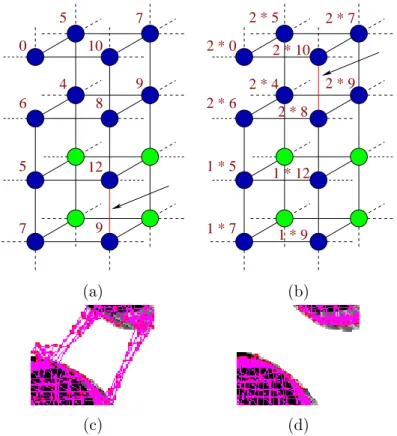
The cubic topology is the straightforward extension of a 2D topology formed by squares or rectangles [10, 9]. Figure 2.2 shows a 4×4×3 TAV with cubic topology. In 3D, the external nodes are on the mesh surface, whereas the internal holes are inside the mesh.

The cubic mesh defines a neighborhood where an internal node has 6 neighbors, whereas an external node has 3, 4 or 5 neighbors according to its location on the corner, edge or face of the mesh, respectively.

2.2.2 Energies

Independently of the mesh topology, the TAV model is defined parametrically as v(r, s, t) = (x(r, s, t), y(r, s, t), z(r, s, t)) where (r, s, t) ∈ ([0,1]×[0,1]×[0,1]). The state of the model is governed by an energy function defined as follows:

(37)

2.2. Topological Active Volumes 19

Figure 2.2: A 4×4×3 cubic mesh. The blue nodes represent the external nodes and the green nodes are the internal nodes.

whereEint stands for the internal energy and Eext is the external energy.

Internal energy objectives Like the 2D model, the internal energy controls the shape and the structure of the net and its calculus depends on first and second order derivatives, which control contraction and bending, respectively. In 3D, the internal energy is defined by:

Eint(v(r, s, t)) = α(|vr(r, s, t)|2+|vs(r, s, t)|2+|vt(r, s, t)|2)+

β(|vrr(r, s, t)|2+|vss(r, s, t)|2+|vtt(r, s, t)|2)+

2γ(|vrs(r, s, t)|2+|vrt(r, s, t)|2+|vst(r, s, t)|2)

(2.10)

where subscripts represent partial derivatives and α, β and γ are coefficients that control the smoothness of the mesh.

In order to compute the energy, the parameter domain [0,1]×[0,1]×[0,1] is discretized as a regular grid defined by the internode spacing (k, l, m) and the first and second derivatives are estimated using the finite difference technique in 3D. Specifically, the first order derivatives are computed using the forward and backward differences as follows:

|vr|2 =

kd+rk2+kd−rk2

2 |vs|2 =

kd+

sk2+kd−sk2

2 |vt|2 = k

d+_t k2+kd−_tk2 2

(38)

The finite difference technique is also used for computing the second order deriva-tives:

External energy objectives Eextrepresents the features of the scene that guide

the adjustment process and is defined as follows:

Eext(v(r, s, t)) = ωf[I(v(r, s, t))]+

where ω and ρ are weights, I(v(r, s, t)) is the intensity value of the original image in the position v(r, s, t),f is a function related to the image intensity, andℵ(r, s, t) is the neighborhood of the node (r, s, t). Thus, given that the repeated polyhedron in the mesh defines the node neighborhood, the shape of the polyhedron influences not only the flexibility of the mesh, but also the way the nodes are adjusted to the objects.

(39)

2.3. Greedy methodology 21

where, again: ξ,̺ are weighting terms, Imax and Gmax are the maximum intensity

values of imageIand the gradient imageG, respectively,I(v(r, s, t)) andG(v(r, s, t)) are the intensity values of the original image and the gradient image in the node positionv(r, s, t),I(v(r, s, t))_nis the mean intensity in an×n×nvoxel neighborhood, his an appropriate scaling function multiplying once again the energy termIO, and GD(v(r, s, t)) is the gradient distance, i.e., the distance from the node position v(r, s, t) to its nearest edge, and the components IODare defined as in the 2D case. Otherwise, if the objects to detect are dark and the background is light, the energy of an internal node will be minimum when it is on a point with a low grey level. On the other hand, the energy of an external node will be minimum when it is on a discontinuity and on a light point outside the object. In this situation, the functionf is defined as:

where the symbols have the same meaning as in equation 2.15.

2.3 Greedy methodology

Most of the minimization techniques are based on performing several steps with a set of choices in each step. Thegradient methods [71], the dynamic programming [12] or the simulated annealing [53] techniques are examples of algorithms that explore the search space iteratively. In this sense, aGreedy algorithm selects the best local solution at each step of the minimization process.

The local choices provide a compromise that produces acceptable approximations and, sometimes, leads to the global minimum solution [27].

A greedy algorithm is a simple minimization method, usually quite efficient and suitable for problems where the choice at every step can produce an optimal solution, i.e., a solution that minimizes the objective function.

(40)

optimizations should converge to an optimal solution. Also, since the external nodes should be on the surfaces, whereas the internal nodes should be inside the objects, a simple initialization strategy is to create a mesh with a homogeneous distribution of nodes within the limits of the whole image. This way, the minimization process will shrink the mesh and will lead the nodes towards the objects of interest.

Then, the energy of the model is minimized using the greedy strategy. At each step, this algorithm tries to minimize the energy functions locally. The mesh energy is computed as the sum of the node energies. Since the greedy strategy performs a local search, the node energy is computed in the current node position within the image and in its neighboring positions. After that, the image position with the lowest energy value is selected as the next node position. The new mesh energy is the sum of the lowest local node energies. These steps are repeated until the mesh energy remains unchanged.

2.3.1 Topological changes. Link cutting procedure

The size and shape of the mesh are established at the beginning of the segmenta-tion process. However, the shape of the object could vary drastically and the final segmentation results could not be as good as possible. Topological changes could be performed in particular areas of the shape with special concavities or irregularities where a better segmentation can be obtained.

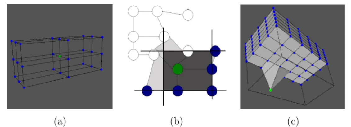
The greedy method introduces a mechanism called link cutting procedure that is applied to the model when the segmentation cannot be improved. It is based on removing a connection between two wrongly located nodes in the mesh by a previous identification of the external nodes wrongly located. Hence, the flexibility of the mesh in this areas will be increased, and the net will be able to improve the adjustment. These nodes wrongly located are the nodes more distant to the object edges. To this aim we use the Tchebycheff’s theorem. This way, an external node vext is wrongly placed if its gradient distance fulfills the following inequality:

GD(vext)> µGD+ 3σGD (2.17)

where µGD is the average gradient distance of the whole set of external nodes and

σGD is their standard deviation.

(41)

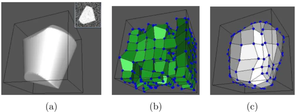
(a) (b)

Figure 2.3: 3D link cutting example. Conversion of internal nodes in external ones. (a) Before the breaking and connection to be removed. (b) Result after the breaking. Green and blue nodes represent the internal and the external nodes, respectively.

of a connection is shown in Figure 2.3, where some internal nodes become external ones after the breaking.

The process of breaking implies a restriction: the squared structure in 2D and the cubic one in 3D of the model has to be preserved, that is, all the nodes and connections has to perform squares or cubes, respectively. The situation of nodes and connections isolated is not allowed. Under this circumstance, sometimes a breaking of a connection implies breaking the topology of the model, that is leaving connections and nodes isolated, but several simultaneous breaking can preserve the topology of the mesh. For example, in Figure 2.4 we can see an example of a breaking that implies the breaking of other connections.

It also can be used to identify internal nodes wrong located. That could be possible in the case the object has a hole inside of the object. Using the same mechanism we can remove some links to create an internal hole and obtain a better adjustment in this part of the object. This mechanism detailed in [11], was not used in the current work, where we only used the link cutting procedure in the external nodes, together with the automatic net division explained next.

2.3.2 Automatic mesh division

(42)

b

a

b a

c d

(a) (b)

Figure 2.4: 3D multiple breaking example. The marked connections has to be removed because: (a) The breaking of connectionaimplies that connectionbdoes not belong to any cube. (b) If any of these connection is removed, the other has to be removed as well, because they do not belong to any cube anymore.

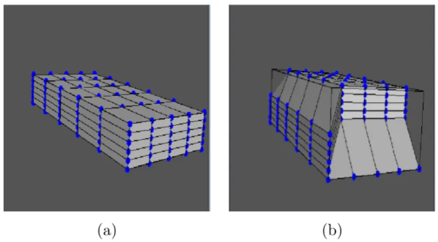
The mesh division is performed by the link cutting procedure. However, this algorithm cannot be applied directly to the automatic division. Since the topology must be preserved, problems arise when cutting a link implies leaving isolated links or planes. In such case, these links cannot be cut so a “thread” composed by squares in 2D or cubes in 3D will appear between two submodels. If one connection in one of these squares or cubes is broken, the topology is not preserved. Figure 2.5 shows these ideas in 2D for a better visualization. Figure 2.5(a) presents an example with a “thread”. Figure 2.5(b) depicts a case that leads to threads. If the labeled link is removed, there will be two threads since no other link can be cut. The 3D case is equivalent.

However, this problem can be overcome if we consider a direction in the cutting process [16]. Thus, a cutting priority is associated to each node whose connection is removed. A higher priority is assigned to the nodes in the cutting direction whereas a lower priority is assigned to the nodes involved in the cut. Figure 2.5(c) shows the recomputation of the node priorities after several cuts in the 2D case. The extension for the 3D case is straightforward. Figure 2.6 also shows a 3D example about how to deal with the link cutting procedure, using priority or not. As we can see, the version that uses priority is able to divide the mesh (Figure 2.6 (d)), meanwhile the one without priority gets stacked leaving threads between both sub-meshes (Figure 2.6 (c)).

(43)

Figure 2.5: Threads and cutting priorities in 2D. (a) Image segmentation with threads. (b) If link “a” is removed, no other link can be removed in order to preserve the TAN topology. (c) Recomputation of cutting priorities. When a link is broken in a direction, the neighborhood in this direction increases its priorities.

0

(44)

removed consist of two neighboring nodes within this set,n1 and n2, that fulfill:

GDvext(n1)×Pcut(n1)> GD(n)×Pcut(n), ∀n6=n1

GDvext(n2)×Pcut(n2)> GDvext(m)×Pcut(m), ∀m6=n2, m∈ ℵ(n1),

(2.18)

where Pcut(x) is the cutting priority of node x, GDvext(x) is the distance from the

position of the external nodexto the nearest edge, andℵ(n1) is the set of neighboring

nodes of n1.

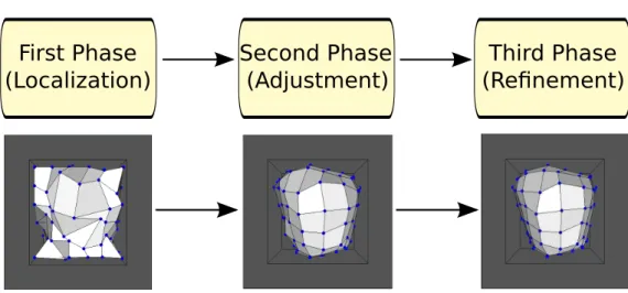
Summarizing, the entire segmentation process including the possible topological changes can be seen in Figure 2.7.

TAM

Figure 2.7: Segmentation process using a greedy strategy diagram.

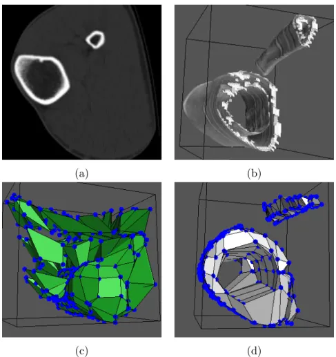
2.3.3 Advantages and disadvantages

(45)

Figure 2.8: Wrong 2D segmentations using the greedy methodology.

However, this method has difficulties in providing acceptable results under com-plex conditions, like noisy images or objects with fuzzy or discontinuous contours. As the method moves the nodes locally to the best neighboring pixel, it is easy to get stacked in noisy regions of the images, falling in local minima. Figure 2.8 shows some results obtained with the greedy local search in some real CT images that presented some artifacts captured that cannot be overcome by the method. The results are not acceptable.

(46)

(47)

Chapter 3

Optimization of Topological

Active Models by means of

Genetic Algorithms

3.1 Introduction

The greedy strategy is a deterministic local search method. Beginning from the same conditions, the method always converge to the same results. The main advantage is that the method provides a result quite fast and direct and requires low memory. However, the method is not capable to reach acceptable results in complex and noisy images. Most of the possible situations in a real domain presents this kind of conditions.

Given the variability of the objects and conditions in the images, it is recom-mended to use a global search method to be able to reach global correct solutions in all the possible situations. There are several global minimization approaches in literature such as the branch and bound algorithms [40], simulated annealing [53], tabu search [36] or evolutionary strategies [37]. The branch and bound algorithms consist of a systematic enumeration of the whole set of candidate solutions by using super and lower estimated bounds of the quantity to optimize. Typically, these tech-niques rely on somea priori structural knowledge about the problem. Thesimulated annealing approach considers, at each step, some neighbors of the current state and decides, given a probability, if the system is moved to the new state or not. It allows non optimal states in the search. This strategy finds a good approximation of the global minimum, but it does not guarantee the global optimum. Thetabu search for-bids states already visited in the search space at least for the upcoming few events.

(48)

30 3. Optimization of TAMs by means of GA approaches

It is similar to the simulated annealing since it accepts new inferior solutions tem-porarily to avoid paths already investigated. Nevertheless, the tabu search selects new states based on their quality, not at random like the previous technique. The evolutionary techniques are based on biological evolution and natural selection laws. The candidate solutions are coded as a population of individuals that are combined and mutated into new individuals (solutions) whose quality is evaluated by means of a fitness function.

In the TAM minimization problem, given that there is no a priori knowledge about the minimum of the energy functions, the use of a branch and bound algo-rithms is not suitable. Moreover, other optimization techniques such as thesimulated annealing or the tabu search are based on a probabilistic local search and could not reach the global minimum. Therefore, an evolutionary technique, with a simultane-ous search over the points of the search space represented by the individuals of the population, may be a complementary approach to find the global minimum in the segmentation process we are dealing with.

3.2 Adapted Genetic Algorithm

Genetic Algorithms (GA) [42, 37] are a particular type of evolutionary techniques broadly applied to optimization problems. The use of a GA in a minimization process requires the definition of a set of characteristics that are defined below.

Genotypic encoding The genetic algorithms require that the set of variables or parameters to be optimized in a specific problem have to be coded in a chro-mosome. Each chromosome, genotype or individual represents a candidate solution of the problem and consists of a set of genes that encodes the opti-mization parameters. Thus, we can represent possible solutions in the entire search space as individuals that compose a genetic population. In our method, each genotype is represented by the list of the coordinates of all the nodes of the mesh. Thus, the chromosome is composed by a list of integers:

x1, y1, z1, x2, y2, z2, ..., xn, yn, zn (3.1)

wherenis the number of nodes in the mesh, andzis the third coordinate only considered in 3D segmentations.

(49)

3.2. Adapted Genetic Algorithm 31

is represented by a given individual. As we explained before, the model has an energy associated that represents how good or bad is the adjustment with respect to the objects in the scene. Thus, the fitness function is the inverse of this energy:

F = 1/E(v) (3.2)

where E(v) is the energy of the mesh described in Equations 2.1 and 2.9.

3.2.1 Evolutionary process

After the definition of the two main terms of an evolutionary method, that is, the genotypic encoding and the fitness function, we can proceed with the definition of the evolutionary segmentation process.

The main steps in a standard GA evolutionary process are depicted in Figure 3.1, and basically consist of the following:

Initial population The first step is the production of the initial chromosomes. These chromosomes are randomly initialized in the search space, conforming the initial population of the evolutionary process. In our application, it means that each individual would be placed in a random part of the image, having all the nodes equidistant among them, as shown for instance in Figure 3.2.

Fitness assignment The quality of the individuals is evaluated using the fitness function. This fitness represents the quality of the possible solution that rep-resents the individual. As we said, the inverse of the energy is used as the fitness function.

Termination condition It is checked to determine the end of the evolutionary process. In particular, if we reach a desirable segmentation or the maximum number of generations is reached, the process finishes.

Selection of individuals for reproduction Two individuals from the popula-tion are selected from the entire populapopula-tion, normally depending on their fitness. There are plenty of possibilities for the selection. We use tourna-ment window selection, that selects a random set of individuals and picks the best individual within this set.

(50)

32 3. Optimization of TAMs by means of GA approaches

and otherad hocoperators. The offspring are introduced in the new generation of the population. Both steps of selecting and producing new individuals are repeated, until the population is filled (using a constant size of the population). Finally, we go to the fitness assignment step, starting again the procedure.

Maximum Generations or

Optimum Result?

No

Yes

End Generation of Initial Population

Assign Fitness to All Individuals

Selection of Two Parents

Crossover and Genetic Operators

New Population

Figure 3.1: Standard genetic algorithm process.

Other important issue in an evolutionary algorithm is the population size. It has to be high enough to preserve the genetic diversity, that is, to cover properly the search space, but it has also not to be too high in terms of computational requirements. Elitism is also introduced in the method. It means that the best individual of each generation is directly copied to the next generation. With elitism, we guarantee the preservation of the best temporal result over the generations.

3.2.2 Genetic operators