Numerical simulation of the evolution of viscous rotating drops

Rotating Drops

Marco A. Fontelos1, Víctor García-Garrido1and Ultano Kindelán2

1_{Instituto de Ciencias Matemáticas (ICMAT, CSIC-UAM-UC3M-UCM), Madrid, Spain.}

2_{Dept. de Matemática Aplicada y Métodos Informáticos, UPM, Madrid, Spain.}

1 _Introduction

2 _{Numerical Method (BEM)}

3 _{Numerical results}

Introduction

Background

Studies concerning the evolution of rotating drops date back to the original experiments of J. Plateau in 1843.

Brown & Scriven (1980) determined branches of solutions where the axial symmetry of the drop is broken and drops present a 2-fold, 3-fold or in general n-fold symmetry.

The branches of solutions with n-fold symmetry contain also solutions such that each lobe consists of a chain of small droplets connected by thin filaments as demonstrated by Heine (2006).

Although there is a huge wealth of equilibrium shapes, one cannot expect that all of them come up to be stable.

Once a rotating drop in equilibrium destabilizes, there are essentially two possibilities:

1 _{Transition towards another equilibrium shape.}

2 _{Evolution in such a way that its surface becomes non-smooth at}

some time and a singularity develops.

In this work we implement a boundary element method to compute theevolutionof drops rotating around a fixed axis, determine the

Equations

Two viscous incompressible fluids: drop & surrounding media.

Fluid drop: µ1,ρ1,u(1),p(1).

Outer fluid: µ2,ρ2,u(2),p(2).

Both fluids are rotating around a common axis with angular velocityω.

Non-inertial frame

ρi

u(_ti)+u(i)· ∇u(i)=

−∇p(i)_+µ

Boundary conditions

Balance of stresses across the interface of both fluids:

T(2)−T(1)

n=2γκn on∂D(t) , (1)

T(k)_{is the stress tensor inside (k =1) and outside (k =2) the drop,} given by:

T_ij(k)=−p(k)δij+µk





∂u_i(k) ∂xj

+∂u

(k)

j ∂xi



 , k =1,2. (2)

Kinematic condition:

vN =u·n≡u(1)·n=u(2)·n on∂D(t) , (3)

Scaling

If the axis of rotation is fixed:

ω×(ω×r) =−ω2rer⇒ρiω2rer=∇

1 2ρiω

2_r2

,Π(i)=p(i)−1

2ρiω

2_r2_.

Characteristic lengthl, typical velocityU(ωl) and a characteristic time scaleτ =l/U:

u(i)= u

(i)

U ,r= r l,t =

t τ,Π

(i)

= l µUΠ

(i)_,ω=ω

bz , µi = µi

µ, ρi = ρi

ρ.

(Re= ρUl_µ ,Ek = _ρωlµ2)

ρiReu(_ti)+u(i)· ∇u(i) = −∇Π(i)+µi∆u(i)− 2 Ekbz×u

(i) _inD

i(t),

Stokes system

T(2)−T(1)n= 1

Ca

2κ−Bo

2 r

2

non∂D(t). (5)

Ca= µU

γ , Bo=

(ρ1−ρ2)ω2l3

γ .

Dealing with the limit in whichRe1 andEk 1, so that viscous forces dominate over inertial and Coriolis forces, we can approximate Navier-Stokes equations by the Stokes system:

Numerical Method (BEM)

Boundary integral formulation of the Stok. syst (6) with b.c. (5)

uj(rp) = − 1

4π

1

µ1+µ2

Z

∂D(t)

fi(r)Gij(r,rp)dS(r)

− 1

4π

µ2−µ1

µ2+µ1

Z

∂D(t)

ui(r)Tijk(r,rp)nk(r)dS(r) (8)

Gij(r,rp) = δij |r−rp|+

(ri−rp,i)(rj−rp,j)

|r−rp|3 , i,j,k =1,2,3, (9)

Tijk(r,rp) = −6

(ri−rp,i)(rj−rp,j)(rk −rp,k)

|r−rp|5 , i,j,k =1,2,3,(10)

fi(r) =

2κ(r)−1

2Ω

2_r2

Procedure for solving the integral equation

1 _{Calculate the curvatureκin each node of the mesh.}

2 Calculate the velocity by obtaining the balance force termffrom

the centrifugal force andκ, replacing it in (8) and solving the resulting integral equation.

3 _{Given the velocityu, we move the points of the surface using the}

explicit Euler scheme.

Numerical results

Initial configuration

Mesh

Elements≈1000 - 20000, Nodes≈500 - 10000

Two families of numerical tests

1 _{Ω =cte. (Ω =}

√ Bo).

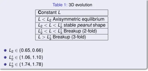
Table 1: 3D evolution

ConstantL

L<L2Axisymmetric equilibrium

L2<L<L∗2stablepeanutshape

L∗₂<L<L∗₃Breakup (2-fold)

L>L∗₃Breakup (3-fold)

L2∈(0.65,0.66)

L∗₂∈(1.06,1.10)

Evolution of the rotating drop at constantLforL=1.41,µ1=1 and

µ2=0.01.

-1 -0.5 0 0.5 1 -0.8 0 0.8 0.4 0.4 -0.4 -0.3 -0.2 -0.10 0.1 0.2 0.3 0.4 x y z

(a) t=2.36

-1 -0.5 0 0.5 1 -0.8 0 0.8 0.4 0.4 -0.4 -0.3 -0.2 -0.10 0.1 0.2 0.3 0.4 x y z

(b) t=8.11

-0.4 0 0.4 -1.5 -1 -0.5 0 0.5 1 1.5 -0.4 -0.3 -0.2 -0.10 0.1 0.2 0.3 0.4 x y z

(c)t=12.36

-0.40 0.4 -2 -1.5 -1 -0.5 0 0.5 1 1.5 2 -0.4 -0.2 0 0.2 0.4 x y z

Shape of the rotating drop at constantLnear the breakup point for

L=3.54 andµ1=µ2=0.5. Observe that forL>L∗3the dominant

mode driving the symmetry-breaking instability is 3-fold.

-2 -1.5

-1 -0.5

0 0.5

1 1.5 2

Different equilibrium or breakup configuration starting from a torus. 0.4 0 -0.4 0.8 -0.8 -0.4 0 0.4 0.8 -0.8 -0.4 -0.2 0 0.2 0.4 x y z

(e) Toroidal initial configuration

-0.4 0 0.4 0.8 -0.8 0.3 0 -0.3 -0.6 0.6 -0.3 -0.2 -0.10 0.1 0.2 0.3 x y z

(f) Equilibrium shape (L=0.85)

0 0.4 -0.4 -0.4 0 0.4 0.8 -0.8 -1.2 1.2 1.6 -1.6 -0.4 -0.2 0 0.2 0.4 x y z

(g) Near break-up (L=1.7)

-1 -0.5 0 0.5 1 -1.5 -1 -0.5 0 0.5 1 1.5 2 -0.20 0.2 x y z

Conclusions

In this contribution we have studied the evolution of rotating viscous drops.

We have developed a numerical algorithm based on the boundary integral formulation of Stokes system.

The numerical algorithm is adaptive and introduces automatically local refinement in the critical regions such as necks, where the drop is going to break up.

Based on the numerical results and the analysis of the equations, we have described the evolution at constant angular momentum