COVID-19 mortality prediction using deep neural networks

During this thesis, a research and comparison was made of modern articles and models aimed at predicting the behavior and development of COVID-19 patients and the disease itself. This research project proposes the use of machine learning models to predict the mortality of COVID-19 patients using as input characteristics of the patients such as vital signs, biomarkers, comorbidities and diagnostics.

Introduction

Motivation
Problem description
RESEARCH QUESTIONS 3 Another situation that is faced is that health care providers are facing severe staffingAnother situation that is faced is that health care providers are facing severe staffing
Research Questions
Solution overview
Main contribution
Literature Review
LITERATURE REVIEW 7 efficient medical resources
LITERATURE REVIEW 9 of the population per day. The metrics utilized to compare the results are Mean Absolute Er-
LITERATURE REVIEW 11 Table 2.1: Comparison of mortality risk models
E+05 and RMSE =
LITERATURE REVIEW 13

In the first months of the pandemics, a shortage of PPE occurred due to the increasing demand, panic buying, hoarding and misuse. A comparison was made with state-of-the-art models such as Random Forest (RF) and eXtreme Gradient Boosting (XGBoost). For the rest of the countries, Italy has better results than the United States.

The time window for the data is from January 2020 to June 2020 with data from countries around the world.

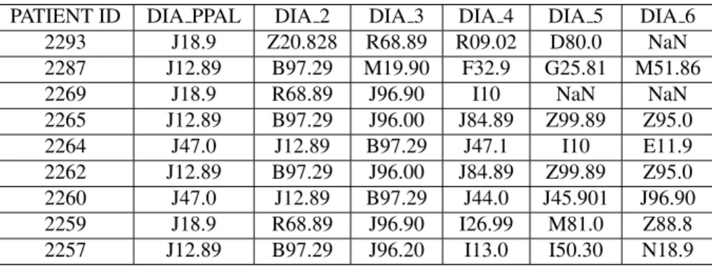
Database

Description
SHapley Additive exPlanations
HM AND HSJ DATABASE 17
HM and HSJ Database

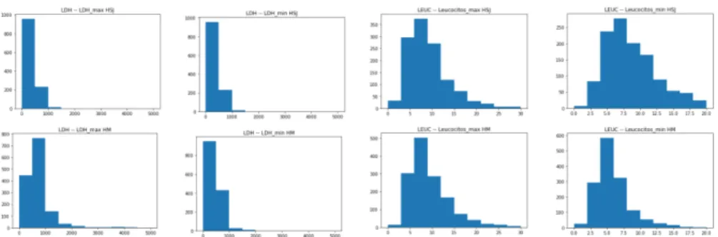
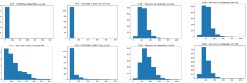
An image of the distributions before normalization of each attribute can be observed on Figures # 3.2-3.8. The tone of the color shows whether the value of the attribute is high or low. In Figure # 3.4 the distribution of the oxygen saturation at admission can be observed, it can be seen that in the HSJ hospital dataset there is a greater variation of values compared to those in the HM Hospitals, tending to almost all of them tended to 100.

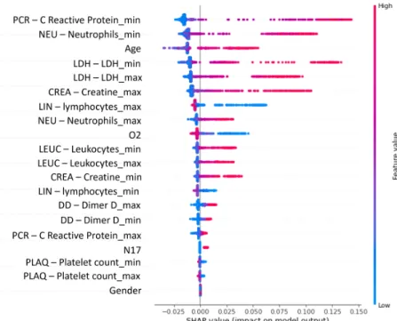
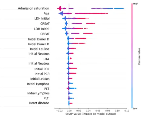
On Figure # 3.6, the distributions of the biomarker LDH are very similar across both data sets, but in the Leukocyte count the biomarker presents a greater spread and variation of values over the range of 0 to 30 than in the HM Hospitals data set. SHAP graphs were created from the HM and HSJ databases; in Figure # 3.9 the results of the SHAP algorithm can be observed using the HM dataset and in Figure # 3.10. By analyzing these two SHAP graphs, the importance of each of the features obtained from the SHAP algorithm can be observed.

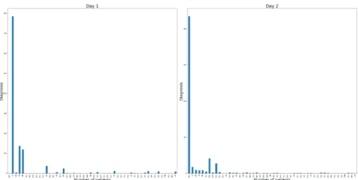
It can be observed on Figure # 3.9 the ranking of the characteristics in descending order, starting with the PCR minimum number, Neutrophil min number, Age, LDH minimum and LDH maximum. The dynamic model is based on the use of the diagnosis information of the patients through time. It was found that the best results of the model were obtained using 50 features (the 50 diagnoses with more frequency throughout the days).

Models

Static model

Train - test split
Deep Learning approach
XGBoost approach

STATIC MODEL 27

Random Forest approach

Dynamic model

Recurrent neural networks

DYNAMIC MODEL 29
MODEL PROPOSAL - STATIC AND DYNAMIC MODEL COMBINATION 31
Model proposal - Static and Dynamic model combina- tion

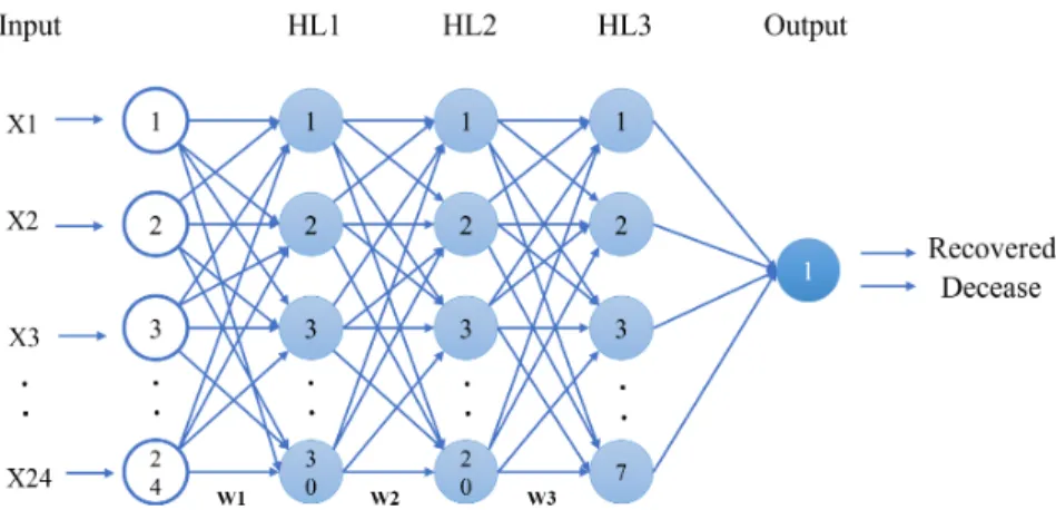
The activation functions can be linear or non-linear, and there are also weights associated with each of the neuron's inputs (represented by w in Figure 4.1). They use multiple ML algorithms to obtain a better model; an analogy of using different trees for this purpose can be seen in Figure 4.3. The output of the RF regressor is the mean or mean prediction of the individual trees.

Some of the variants of the common RNN that were created to solve this problem are the LSTM and the GRU. LSTM is characterized by the use of cell state, which is responsible for enabling information flow with linear interactions. The output is determined by h_t, which is the output of the current network, and c_t, the memory of the current unit.

GRU is characterized by combining the gap and input ports into a single update port, and merges the cell state with the hidden state. A sensitivity analysis was performed to obtain the factor values for the percentage with the best results. The results of the sensitivity analysis can be found in appendix .6. The overall flow of the logic in the second model approach can be observed in Fig.

Results

First model approach - Deep Learning

HM database

FIRST MODEL APPROACH - XGBOOST 35

HSJ database

First model approach - XGBoost

HM database
HSJ database

First model approach - Random Forest

HM database
HSJ database

GENERAL COMPARISON OF RESULTS 37
General comparison of results
Second model approach - LSTM individual results
Static and Dynamic model combination results
DISCUSSION 39
Discussion

Table # 5.2 presents the results of the DL model run by training with the HM hospital dataset and testing with each of the different datasets (HM, HSJ and CEM), column model shows which model was used, training and test dataset columns represent which databases were used for training and testing, and the shape of training and testing represents the proportions of training and testing datasets (number of patients and number of features). The column Model represents which model is used, as previously shown in the HM database example, and the remaining columns represent the results for each metric. It can be observed that the results obtained are lower than those obtained with the HM database in the case of cross-validation and that the average value of 4 trials is around 0.6.

Table # 5.4 presents the results of the DL model trained with the HSJ database and using the HSJ, HM and CEM databases for testing. The rest of the columns show the results of the benchmarks for each of the iterations. This table presents the comparison of three runs of the RF model with the difference of change in the test data set used.

For the first case HM Hospitals were used for training and testing, the shape of the distributions is presented in the shape and shape test columns, and in the rest of the columns the results for the metrics can be seen. When using a different distribution, the scores on the MPCD drop to about 0.5 and the rest of the metric drops as well. Further tests with different values on the hybrid model formula can be seen in Table # 5.13 and Appendix .6.

Conclusions

Contributions
Limitations
Future work
Acknowledgement
PUBLICATIONS 43
Publications

One of the main limitations during the development of this thesis was the availability of more complete historical and reliable data from patients with COVID-19. The amount of historical data was limited for the dynamic model case in the HM Hospitals database and in the other two databases used. there were no dynamic features to work with. For the static model, the number of patients with a complete file was also limited by the time of start and development of the project; it was only available in one of the databases the project was developed with for training and testing. Another limitation is that the proposed model does not take into account the recent cases of already vaccinated patients and how this vaccination affects the development of the disease and the final prediction of the model.

The research and models created during this work with the historical data and characteristics of the patients can be used in the future as a basis for many more different purposes of prediction, such as a more specific level of development of the disease in COVID- 19, or even with another die using the same kind of logic in the preprocessing and treatment of data and minor changes in architecture and characteristics of the patients. The combination of the static and dynamic models can also be used as a basis for the creation of more models for different purposes of prediction, such as the mortality of patients with diseases. Rub'en Morales Menendez for his great support and guidance during this path of the Master.

I would like to thank Amazon for their contribution to the development of a web application I worked on during my studies that used some of the models created during this research. Etna Rojas for support at the beginning of the research and during the development of the project. My friends, especially those who were present during this master's period, brought me moral support and even ideas for daily work.

1. ACRONYMS DEFINITIONS 45

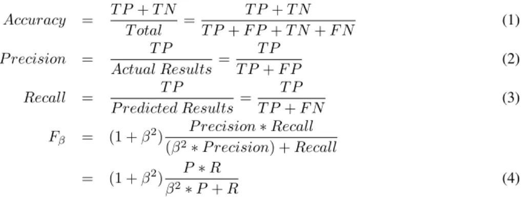
The Confusion Matrix (CM) can be used to report results in classification problems, because it is possible to observe the relationship between the classifier's results and the true results, Figure #2. the diagonal one represents the mis-classified ones; when an asymmetric CMis can reveal a biased classifier. Accuracy is a metric used to predict the accuracy of an ML model, eqn (1). Accuracy means the percentage of results that are relevant, equation (2). Recall refers to the percentage of the total number of corresponding results correctly classified, equation (3) . The area under the AUC curve of the receiver operating characteristic (ROC) curve is a good point to evaluate the real classification performance of a model.

This curve is obtained by measuring the TP rate (TPR) and FP rate (FPR) using different decision thresholds. The closer the AUC score is to 1, the better the prediction performance of the model. The Maximum Probability of Correct Decision (MPCD) is a probability-based measure of classification performance aimed at analyzing highly unbalanced data structures.

TheMPCDis a probabilistic measure of classification performance – powered by detection – that is highly sensitive to FNin highly/ultra unbalanced classes.

3. OCTM ALGORITHM 47

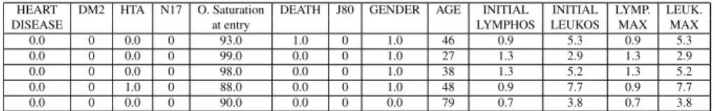
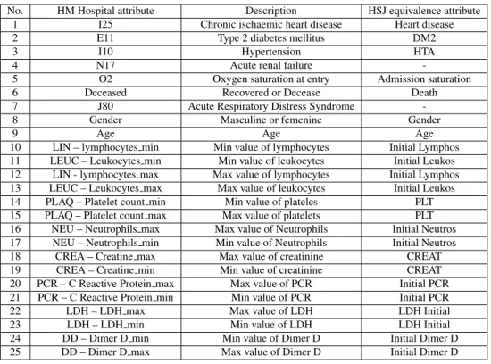
10 LIN – lymphocytes min Min value of lymphocytes Initial Lymphosis 11 LEUC – Leukocytes min Min value of leukocytes Initial Leukosis 12 LIN - lymphocytes max Max value of lymphocytes Initial Lymphosis 13 LEUC – Leukocytes max Max value of leukocytes Initial Leu. 16 NEU – Neutrophils max Max value of Neutrophils Initial Neutros 17 NEU – Neutrophils min Min. value of Neutrophils Initial Neutros. 20 PCR – C Reactive protein max. Max. value of PCR Initial PCR 21 PCR – C Reactive protein min Min. value of PCR Initial PCR.

5. DYNAMIC MODEL HYPERPARAMETER AND PARAMETER EXPERIMENTATION AND RESULTS49

6. SENSIBILITY ANALYSIS IN MIXED MODEL RESULTS 51

An elevated level of c-reactive protein may be an early indicator to predict the risk of covid-19 severity. Machine learning prediction of mortality in patients diagnosed with COVID-19: a Korean nationwide cohort study. Prediction of covid-19 using deep recurrent neural networks (rnns) with closed recurrent units (grus) and long short-term memory (lstm) cells. Chaos, solitons and fractals.

Prediction of respiratory decompensation in covid-19 patients using machine learning: The ready trial.Computers in Biology and Medicine. Covid-19 mortality prediction for India using statistical neural network models. Frontiers in Public Health(2020), 441. Machine learning-based early warning system enables accurate prediction of mortality risk for covid-19. Nature communication.

Prediction of mortality risk in patients with covid-19 using artificial intelligence to aid medical decision making. MedRxiv (2020). Mortality prediction model for the triage of Covid-19, pneumonia and mechanically ventilated icu patients: A retrospective study. Annals of Medicine and Surgery. Time series prediction of covid-19 using deep learning models: India-US comparative case study.Chaos, Soliton and Fractals.