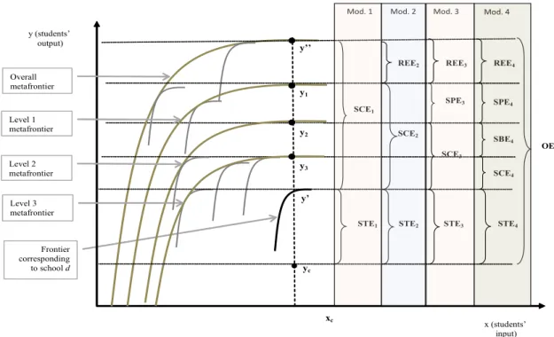
In other words, the proposal of Thanassoulis and Silva Portela (2002), because it does not take into account the resources allocated to each school, could be influenced by a possible overestimation of the effect of the school. We will also refer to model 2, or to the decomposition in (3) as the tripartite decomposition of the school's overall efficiency. In the case of expression (5), we will refer to it as the four-part decomposition of the school's overall efficiency.

The order- m estimation of the frontier efficiency coefficients
Given the importance of this literature, we will closely follow the approach used by McEwan (2001), which is very similar to that used by Mizala and Torche (2012), who considered the two-stage selection bias correction devised by Lee ( 1983). to choose between several alternatives, where the first step is a choice model in which the dependent variable is the type of school the student attends—in our case, four types of schools. Lee (1983) for choosing among several alternatives, where the first step is a choice model in which the dependent variable is the type of school the student attends—in our case, four types of schools.
The order-m estimation of the frontier efficiency coefficients
We will provide all data on the estimation of this selection bias effect in section 3. Selection bias effect (SBO): This effect captures the impact caused by the fact that more able, motivated or ambitious students can select themselves into a specific type of school.
The order-m estimation of the frontier efficiency coefficients
Documento de Trabajo – Núm which are drawn from the conditional distribution of the output matrix Y respecting the condition . j c j As m increases, the number of observations considered in the estimation approaches the observed units satisfying the condition ym,j >yc,j, and the expected m-order estimator in each of the iterations b α~cb tends to the FDH efficiency coefficient α ~cFDH. To adapt the estimation process to this situation, as previously discussed in models 2, 3 and 4, here we define a multilevel frontier estimation. y1,j,ym,j), which are drawn from the conditional distribution of the output matrix Y respecting the condition ym,j >yc,j.
As m increases, the number of observations considered in the estimation approaches the observed units that satisfy the condition ym,j >yc,j, and the expected order-m estimator in each of the b iterations α~cb tends to the efficiency coefficient FDH α~cFDH . As m increases, the number of observations taken into account in the estimation approaches the observed units that satisfy the condition ym,j > yc,j, and the expected estimator of order m in each of the b iterations α~cb tends to the efficiency coefficient FDH α~cFDH . To adapt the estimation procedure to this situation, as previously discussed in models 2, 3, and 4, we define multilevel marginal estimation here. tends to the efficiency coefficient of FDH. y1,j,ym,j) which are drawn from the conditional distribution of the output matrix Y subject to the condition ym,j > yc,j.
To adapt the evaluation process to this situation, as discussed earlier in Models 2, 3 and 4, we define here a multilevel frontier assessment. coefficients, depending on the level of m. y1,j,ym,j), which are derived from the conditional distribution of the output matrix Y with the condition ym,j >yc,j. As m increases, the number of observations considered in the estimate approaches the observed units satisfying the condition ym,j >yc,j, and the expected order-m estimator in each of the bititerations α~cb tends to the FDH efficiency coefficient α~cFDH.
Data Description and Sources
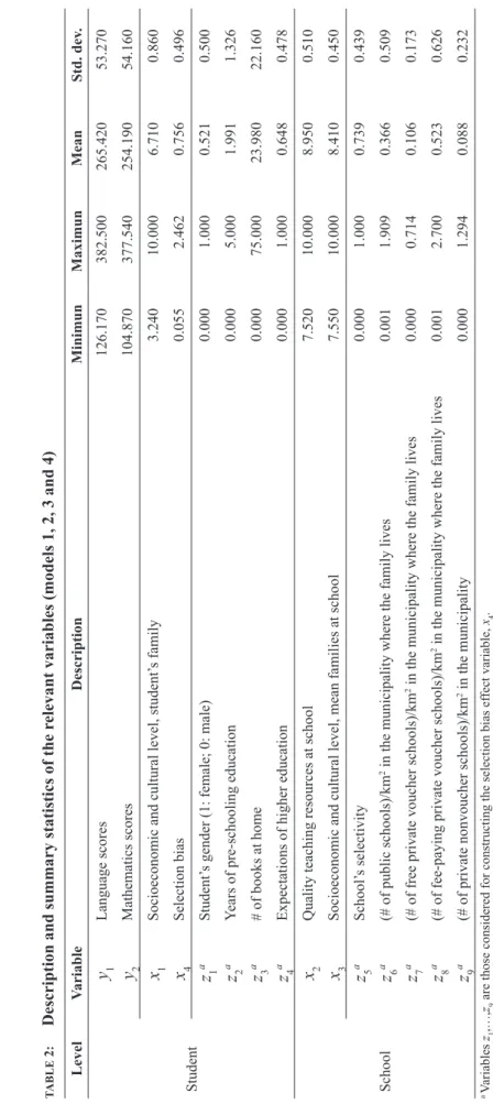
The variables were obtained using the questionnaire answered by the parents of students participating in the SIMCE. At the school level, the variable "availability of quality teaching resources in the school" (x2) corresponds to a latent variable consisting of five questions drawn from the questionnaire answered by the teachers. In our specific application, the Zc,d values considered in the estimation of equation (11), corresponding to the student level, are: (i) gender (1: female; 0: male); (ii) number of years of pre-school education; (iii) number of books at student's home; (iv) expectations of parents on the educational level that can be achieved by their children (1: the expectations are to achieve higher (university) education; 0: otherwise).
Those corresponding to the school level are: (v) school selectivity, which is a dichotomous variable that takes the value 1 when at least 50% of the school's parents should meet one of these criteria when (12). Those corresponding to the school level are: (v) school selectivity, which is a dichotomous variable that takes the value 1 when at least 50% of the school's parents would meet one of these criteria, when. Those corresponding to the school level are: (v) school selectivity, which is a dichotomous variable that takes the value 1 when at least 50% of the school's parents had to meet one of these criteria when enrolling their children in the school, i.e.
We therefore follow a similar approach to Mizala and Torche (2012), who also use the number of schools (of each type) per square kilometer in the pupil's municipality to control for the supply of schools in different sectors. in the municipality where the family lives (a similar strategy is followed by McEwan, 2001, among others) 9. We therefore follow a similar approach to Mizala and Torche (2012), who also use the number of schools (of each type) per square kilometer in the student's municipality to control the offer of schools from different sectors in the municipality where the family lives (a similar strategy is followed by McEwan, 2001, among others). 9.
Results
To more explicitly take into account the fact that summary statistics can hide some relevant information, we considered some tools that allow a fuller overview of the distributions corresponding to the different components of the considered models. Specifically, using kernel methods, we made estimates of the densities corresponding to each indicator for model 4, i.e. Note: All figures contain densities estimated using the kernel density estimate for the various components of the binomial decomposition in expression (1).
Note: All figures contain densities estimated using kernel density estimation for the various components of the binomial decomposition in expression (1). Analogous to the analysis performed bipartite decomposition (model 1) in figure 5.b, figure 5.c illustrates how the inclusion of the resource endowment effect (REE) affects the relative contributions of each component of the overall efficiency, while the full distributions are taken into consideration. of the effects. As shown in Figure 5.c, the effect of the resource allocations is much closer to the school effect, SCE4, than to the student effect, STE, which contributes modestly to the overall efficiency.
Finally, the contribution of the selection bias effect (SBE) considered by the quinquepartite decomposition to the overall school efficiency is included in figure 5.e. All of them have tight densities, indicating that the effect is homogeneous, while the flatter shape of the density corresponding to the school effect (SCE4) indicates a large degree of heterogeneity across schools.
Conclusions
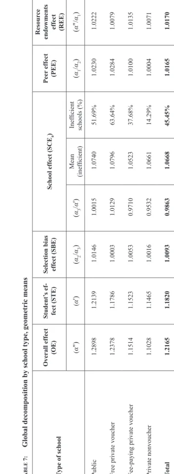
However, and despite controlling for peer, resource endowments, and selection bias effects, public school performance is lower than matched fee-paying private voucher and private non-voucher schools, and the differences are statistically significant. This result does not hold when compared to free private voucher schools, whose performance is statistically lower than that of public schools. Indeed, in comparing public schools and free private voucher schools—both of which compete for similar students—it becomes clear that the global efficiency estimator for public schools averages 1.2898, higher than that of free private voucher schools, whose average is 1. 2378.
However, these differences are not caused by management differences between each school type (1.0015 vs. 1.0129 for public and free private voucher schools, respectively), but rather by other factors, especially those related to student characteristics. Indeed, the average negative effect of REE is more than twice as large in public schools as it is in free private voucher schools, and the peer effect attributable to student characteristics is also significantly greater in public schools than in fee-paying private voucher schools and private non voucher schools. These results strengthen both the view that argues for a separate analysis of the two types of voucher schools, and those others who believe that the fees collected by paying private voucher schools allow important resources to be acquired for the school (in addition to the teaching resources), thereby the differences between public and private education become permanent.
According to the obtained results, it seems that the most important resource is the schools. inefficiency is the resource endowment effect, closely followed by the peer effect. This result is particularly important because it mainly affects public and free private voucher schools, which are unable to collect tuition from families and whose students generally come from the most vulnerable communities in Chile.
This result is in agreement with previous results such as those of Valenzuela et al. 2009), who found that the voucher system has a tremendous effect on the high socioeconomic segregation of the Chilean education system, or Hsieh and Urquiola (2006), who argued that this segregation can be exacerbated by competitive mechanisms to attract students. Evaluating efficiency and productivity research: A review and analysis of the first 30 years of scientific literature in DEA. The Effects of Universal School Choice on Achievement and Stratification: Evidence from Chile's Voucher Program.
An evaluation of the effectiveness of Québec's school boards using the Data Envelopment Analysis method. A comparison of the relationships of community climate and academic climate with mathematics achievement and attendance during middle school. Evaluating the cost-effectiveness of the Italian banking system: What can be learned from the joint application of parametric and non-parametric techniques.
Currently he is responsible for the project Gestión y evaluación de las organizações (Spanish Ministry of Science and Innovation, VI National Scientific Research, Development and Technological Innovation Plan 2008-2011). He has also taught at the University of Alicante and has received scholarships from various institutions (including Fundación Caja Madrid). He has held positions as visiting researcher at the Autonomous University of Barcelona, the University of New South Wales (Australia) and the Department of Economics at Oregon State University (USA).
He has participated in many Spanish and international congresses and is the main researcher in the project under the Spanish national research program Evaluación de la eficiencia.
Documentos de Trabajo
Documentos
Claudio Thieme Diego Prior
Emili Tortosa-Ausina
A Multilevel
Decomposition of School
Performance Using Robust
Frontier Techniques