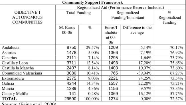
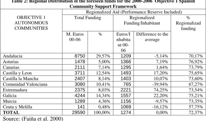
However, in a specific analysis of the Spanish economy, De la Fuente (2003b) points to the important role of structural funds in the growth of the Objective 1 regions and for the whole. In Section 4, the model is simulated to quantify the impact of the CSF measures on the Galician economy. Given that the objective of this document is to assess the medium and long-term effects of the Galicia Community Support in 2000-2006 for the Galician economy.
The production function is assumed to be of the Cobb-Douglas type, supplemented with public capital.
An estimation of the basic model
- General Characteristics
- An estimation of the production function
- An estimation of the demand function for Labour
- An Estimation of the private investment function
The non-agricultural private VSHB in this case consists of the sum of the VSHB for industry (the sum of branches 06 and 30 corresponding to B-6), construction (branch 53) and the retail sector (branch 68 without PISB). All equations to be evaluated are in logarithmic form except for the index for human capital. Corresponding individual effects were included in each of the equations and treated as fixed effects.
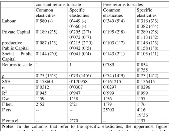
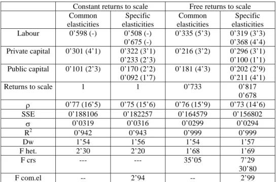
In the next two columns, the return to scale estimate is based solely on the data. In columns 1 and 3 it is assumed that the elasticities of the different production factors are the same for all regions. The data unequivocally reject the hypothesis that returns to scale are constant, and this rejection is particularly unequivocal in the case of Objective 1 regions.
Further, the precision of the estimators is biased when constant returns to scale are assumed, and this is verified by contrasts in heteroscedasticity. The figures given for labor and the two types of capital represent the estimated elasticities (t); returns to scale are the sum of all elasticities; ρ is an estimate of the first-order auto-regressive coefficient; SSE is the sum of squared errors; σ estimate of the standard deviation of the residuals; R2 coefficient of determination; dw statistics Durbin- Watson;. The hypothesis of common elasticities for both groups of regions is just within the limits of acceptability.
The figures for labor and the two types of capital represent the estimated elasticities (t); returns to scale are the sum of all elasticities; ρ is an estimate of the first-order autoregressive coefficient; SSE is the sum of squares of errors; σ the estimate of the typical deviation of the residuals; R2 the coefficient of determination; dw Durbin-Watson statistic;. In column 1 the given elasticity of income is the same for all regions, while in the second column the Objective 1 regions and the rest of the regions were allowed to have different elasticities.
The model augmented with the addition of CSF funds
- CSF aid for infrastructures
- CSF aid for education and re-qualifacation of human capital
- CSF investment aid
- Definitive equation for income in the model with CSF
The introduction of the CSF does not change the exogenous nature of infrastructure investment. Let CSFit be the EU funds allocated for this objective, let rI be the co-financing ratio for the national public sector, defined as the contribution of the domestic public sector for each monetary unit provided by the EU. The question this definition raises is therefore; How could the human capital indicator be changed with EU funds for providing secondary school education to those active residents with only primary school education.
Of course, in practice, part of the funds go to the education of individuals who already possess intermediate studies, which means that the program will not necessarily increase the human capital index as defined in section 3.2.1. This is true because the "real" cost consists of teaching costs along with the opportunity cost associated with lost work hours or a long overtime. It should be noted that, due to the way the indicator is determined, there is no depreciation of the existing capital stock.
Where CSFPFt represents the total amount of public funds designated for the program and rPA/PB is the ratio of the co-financing of the internal public sector destined to support production. Where the induced investment is part of the basic model and is given by the equation. The independent component of private investment provides an additional designation for the final version of the model, which has the following form.
A quantification of the impact of CSF on the Galician economy
General approach
A detailed description of the scenarios .1 Scenario 1: the reference economy
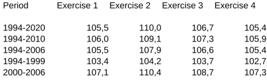
Finally, for the reasons outlined in section 3.2.2, the specifications of the most appropriate production function for the years 1980-1992 may be open to debate. Since different specifications can lead to important differences in the simulated trajectory of the economy, the following sensitivity analysis was performed. By following this methodology, it becomes possible to compare the results and evaluate the extent to which the estimated effects of the CSF program are robust with respect to the specific production function used.
Quantifying the impact of CSF on income compares the results of each of the four exercises. The investigation of the effects of the macroeconomic variables of capital stocks and employment is carried out using the results of the assumptions defined in exercise 1. Internal public co-financing was not treated in the same way due to the variety of potential interventions and the possibility of there are imbalances.
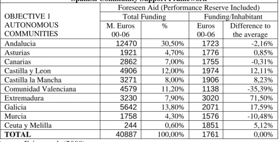
Consequently, the averages of the estimated co-financing ratios were calculated and applied to the relevant EU funds. To estimate the size of the CSF program in relation to the Galician economy, table 9 provides some of the coefficients for the volume of monetary resources involved in this program together with the main regional macroeconomic variables. As in the case of the reference economy, a sensitivity analysis was performed to determine the extent to which certain factors such as returns to scale of the production function could distort the estimate of the effects of the CSF.
Shock estimations
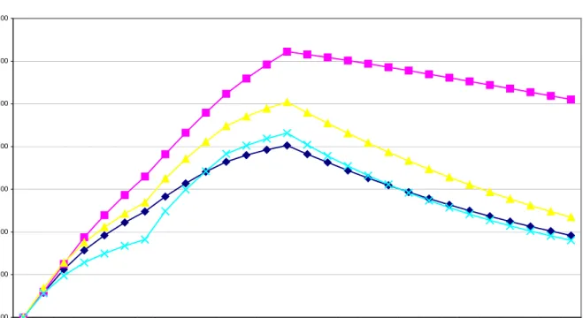
In the long run, however, the strength of the boost to the economy begins to wane and the benchmark economy begins to catch up in three out of four cases. This contribution is measured by taking the difference between the simulated income with CSF funds and the income for the same year for the reference economy, expressed as a percentage of the latter. The real core of interest lies in the fact that these figures deviate from their previous values due to the.
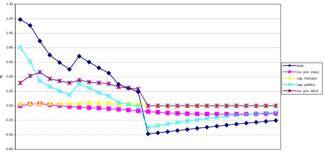
For this purpose, each of the factors for each year for the reference economy is compared with their counterparts in the economy with the ASF and the relative differences in growth are given in graph 3. From the above graph it can be observed that from 2007 onwards the increase in income in the economy with the CSF is actually lower than that of the reference economy due to the significant drop in total investment caused by the finalization of the program. Finally, graphs 4 to 7 show the evolution of the difference in relation to the stock of private capital (graph 4), the stock of public capital (graph 5), the stock of human capital (graph 6) and employment (graph 7).
As in chart 1, for private capital, public capital and employment, the value appearing on the "y" axis for each year and scenario reflects the difference between the value of the variable in the economy with. Subsequently, and after the finalization of the GSR, this difference also begins to decrease, falling to a figure of 3.6% in 2020. The difference with respect to the reference economy does not decrease quite as quickly as with the other variables, given that at the end of the period analyzed, it is still about 3.1% higher than in the case of the economy with CSF.
Conclusions
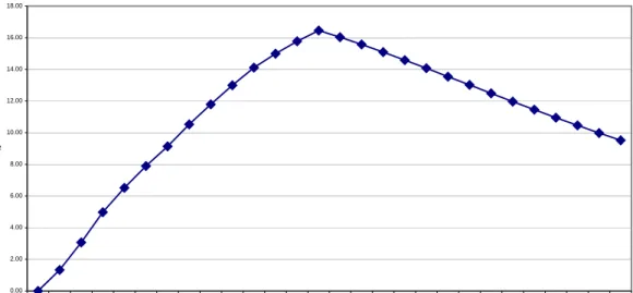
Finally, employment at the maximum deviation is actually just over 5.4% greater than in the case of the economy with FSR, which amounts to 38,700 jobs at constant prices, 6.8% of private nonfarm employment in 1992. On the other side, the cumulative effect of FSRs on the stock of private capital (public capital) exceeds sixteen percentage points (fifteen percentage points) compared to the scenario without FSR. This percentage subsequently falls, but in the longer term it is still more than nine percentage points (three percentage points) higher than in the reference economy.
Given the presumed absence of depreciation, when the difference reaches its maximum, it stabilizes at an estimated figure of around 6.5%.
2003): “Sobre la eficacia de la política regional comunitaria: el caso de Castilla-la Mancha”, Documentos de Trabajo 2003-25, FEDEA. 164/2001 La evolución de la política de gasto de las administraciones públicas en los años noventa Alfonso Utrilla de la Hoz y Carmen Pérez Esparrells. 169/2001 La política de cohesión de la UE ampliada: la perspectiva de España Ismael Sanz Labrador.
172/2002 La investigación en curso sobre la descripción, representatividad y propuestas metodológicas de los presupuestos familiares para la explotación de la información sobre ingresos y gastos. 190/2004 Una aproximación al análisis de los costes de la esquizofrenia en España: modelos jerárquicos bayesianos. Antonio Estache, Beatriz Tovar de la Fé y Lourdes Trujillo 194/2004 Evolución sostenida de los fondos de inversión españoles.
Ana Rodríguez-Álvarez, Beatriz Tovar de la Fe y Lourdes Trujillo 202/2005 Complejidad contractual en alianzas estratégicas. 203/2005 Factores determinantes del desarrollo del empleo en las empresas adquiridas mediante la opa de Nuria Alcalde Fradejas e Inés Pérez-Soba Aguilar. 205/2005 Precio del suelo con presión urbana: un modelo para España Esther Decimavilla, Carlos San Juan y Stefan Sperlich.