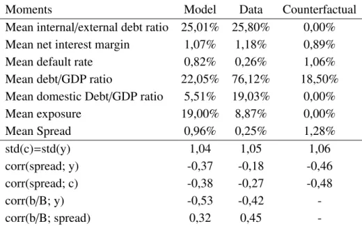
A thorough analysis of recent sovereign debt crises reveals the critical role that demand factors play in the public debt market. This phenomenon is not exclusive to recent crises, as the behavior of sovereign debt holders also played a crucial role in the Latin American debt crisis of the 1980s. Specifically, our model shows how the decline in economic activity, together with domestic bank capital constraints, may lead to an increase in the share of domestic banks in the debt holder base.
The proportion of total debt held by domestic banks varies widely, ranging from 5% in the British Isles to over 40% in the case of the Czech Republic. Before 2008, during the strong economic growth of the early 2000s, there was a gradual reduction in the weight of domestic banks in the debtor base. The share of the domestic banking sector in the base of holders of government debt bonds is negatively correlated with economic activity in developed economies.
As is common in the sovereign debt literature, we assume that the main objective of a benevolent government is to increase household welfare. These transfers and the repayment of existing debt are financed by the state by issuing new debt. Analyzing the other parameters in the multiplier, we notice that it increases with higher values of the capital limitation parameter (ψ).
So, in the interest of all agents, the bank accepts that first small fraction of the debt.

SOVEREIGN DEBT, DEFAULT AND INTERNATIONAL LIQUIDITYLIQUIDITY
At this point, we do not take a position on the source of the ratio or a clear definition of a risk-free asset. In Section 3.4, we present our baseline model, an extension of the baseline model in the strategic default literature. The cross-correlation between our measure of global liquidity and TFP of a small open economy deserves comment.
Clearly, there are important simplifying assumptions in the behavior of the riskless asset question. The parameters that have the greatest impact on the risk-free rate of the model are the average of the liquidity shocks (µw) and the supply elasticity of the risk-free assets (ξ). These results indicate that the simple version of the model falls short of fully replicating the dispersion dynamics observed in the data.
The impact of the risk-free rate on the small open economy operates through two distinct channels. Thus, it should be supplemented by an exogenous correlation between the TFP process of the small open economy and the lenders' wealth process. Moreover, the fall in the global risk-free rate improves the financing conditions of producers of intermediate goods, leading to an increase in the total output of the economy.
This result could not be achieved by the simpler model, with a lack of endogenous production, international investors facing an increasing supply of risk-free assets, and a negative correlation between the economic TFP process and the investor wealth process. In the third sub-sample, we include observations in which investor wealth is within one standard deviation of the mean (Mean). In the fourth sub-sample, we include observations in which wealth is above one standard deviation of the mean but less than two.
We recalibrate the baseline model setting ρzw = 0 to eliminate any exogenous correlation between the outcome and investor wealth. We recalibrate the baseline model setting ξ = 0 to make the supply of the risk-free asset perfectly uniform and therefore the risk-free interest rate insensitive to changes in investor wealth. Thus, we eliminate any exogenous correlation between return and investor wealth, leaving only the endogenous one, and make the supply of the risk-free asset completely uniform, so that the risk-free interest rate does not respond to changes in investors. 'wealth.
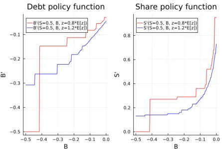
In our model, the supply curve for the risk-free asset is not perfectly elastic, which differs from conventional sovereign debt models. As demand falls, the price of the risk-free asset falls, leading to an increase in the risk-free rate.

PERTURBATING AND ESTIMATING DSGE MODELS IN JULIAJULIA
2006] is one of the first articles to comprehensively compare solution methods for the standard Real Business Cycle (RBC) model. 2018]; and document the gains at different steps of the solution method up to different orders for Julia compared to implementing the algorithm in Matlab. For this reason we use a medium-scale variant of the New-Keynesian model for a closed economy with complete financial markets and capital accumulation.
This model, unlike the case of the NGM, has a larger set of predetermined variables (capital, the cost of price spread, inflation and the nominal interest rate). The equilibrium conditions for this model as well as its notation in terms of the perturbation method are included in the appendix. The notation and structure of this section draws heavily from Schmitt-Grohé and Uribe [2004], as the solution we implement in Julia uses this notation and method to solve the square matrix equation of first order approximation.
We introduce the perturbation parameter as σ, a positive scalar representing the degree of model uncertainty, and denote it by the nx × nϵ matrix. The solution to this problem would be a set of policies that depend on the level of uncertainty of the economy. To implement the solution in Julia, we consider the standard parameterization for both models, shown in table 4.1.
In practice, finding a good density from which to draw the draws, g(θ), is very difficult, and as you can see, this is a key step of the method. Our priors are the truncated normal for the persistence of the technology shock and the inverse gamma for the standard deviation. At this point, a few words about the implementation of the routine in Matlab and Julia are important.
Following the Matlab implementation of the package by Schmitt-Grohé and Uribe [2004], we make extensive use of the symbolic toolbox to obtain the steady-state expressions and derivative matrices of each model in terms of parameters. For the solution phase, Julia is faster than Matlab even without this package, but the package is also available in Julia, including it - which also enhances the matrix handling in Julia - allows us to achieve the benefits shown in the table and will to be responsible for the benefits of the assessment phase. The equilibrium conditions of the New-Keynesian model in its standard form with CRRA preferences are given by,.
BIBLIOGRAPHY