Landau damping
C´edric Villani
Universit´e de Lyon & Institut Henri Poincar´e, 11 rue Pierre et Marie Curie, F-75231 Paris Cedex 05, FRANCE
E-mail address: [email protected]
A MarseilIe, en juillet 2010 `
Contents
Foreword 7
Chapter 1. Mean field approximation 9
1. The Newton equations 9
2. Mean field limit 10
3. Precised results 14
4. Singular potentials 15
Bibliographical notes 17
Chapter 2. Qualitative behavior of the Vlasov equation 19
1. Boundary conditions 19
2. Structure 20
3. Invariants and identities 21
4. Equilibria 23
5. Speculations 24
Bibliographical notes 25
Chapter 3. Linearized Vlasov equation near homogeneity 29
0. Free transport 29
1. Linearization 32
2. Separation of modes 34
3. Mode-by-mode study 35
4. The Landau–Penrose stability criterion 39 5. Asymptotic behavior of the kinetic distribution 44
6. Qualitative recap 45
7. Appendix: The Plemelj formula 47
8. Appendix: Analyticity and regularity 49
Bibliographical notes 51
Chapter 4. Nonlinear Landau damping 53
1. Basic concerns 53
2. Backus’s objection 54
3. Nonlinear time scale 54
4. Elusive bounds 55
5. Numerical simulations 56
3
4 CONTENTS
6. Theorem 56
7. The information cascade 61
8. Scheme for attack 62
Bibliographical notes 64
Chapter 5. Gliding analytic regularity 67
1. Preliminary analysis 67
2. Algebra norms 68
3. Gliding regularity 71
4. Functional analysis 72
Bibliographical notes 73
Chapter 6. Characteristics in damped forcing 75
1. Damped forcing 75
2. Deflection 76
Bibliographical notes 78
Chapter 7. Reaction against an oscillating background 79
1. Regularity extortion 79
2. Solving the reaction equation 80
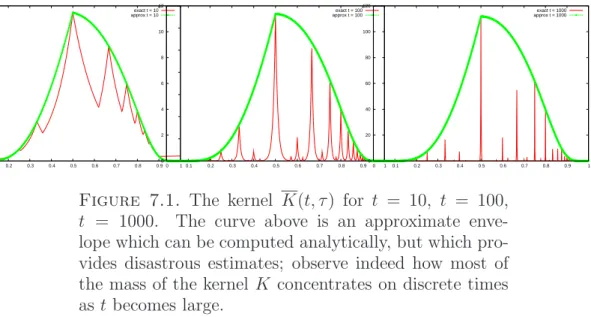
3. Analysis of the kernel K 82
4. Analysis of the integral equation 85
5. Effect of singular interactions 87
6. Large time estimates via exponential moments 89
Bibliographical notes 91
Chapter 8. Newton’s scheme 93
0. The classical Newton scheme 93
1. Newton scheme for the nonlinear Vlasov equation 95
2. Short time estimates 96
3. Large time estimates 98
4. Main result 105
Bibliographical notes 105
Chapter 9. Conclusions 107
Bibliographical notes 109
Bibliography 111
Abstract. This course was taught in the summer of 2010 in the Centre International des Rencontres Math´ematiques as part of a program on mathematical plasma physics related to the ITER project; it constitutes an introduction to the Landau damping phe- nomenon in the linearized and perturbative nonlinear regimes, fol- lowing the recent work [76] by Mouhot & Villani.
5
Foreword
In 1936, Lev Landau devised the basic collisional kinetic model for plasma physics, now commonly called the Landau–Fokker–Planck equation. With this model he was introducing the notion of relaxation in plasma physics: relaxation `a la Boltzmann, by increase of entropy, or equivalently loss of information.
In 1946, Landau came back to this field with an astonishing concept:
relaxation without entropy increase, with preservation of information.
The revolutionary idea that conservative phenomena may exhibit ir- reversible features has been extremely influential, and later led to the concept of violent relaxation.
This idea has also been controversial and intriguing, triggering hun- dreds of papers and many discussions. The basic model used by Landau was the linearized Vlasov–Poisson equation, which is only a formal ap- proximation of the Vlasov–Poisson equation. In the present notes I shall present the recent work by Cl´ement Mouhot and myself, extend- ing Landau’s results to the nonlinear Vlasov–Poisson equation in the perturbative regime. Although this extension is still far from handling the mysterious fully nonlinear regime, it already turned out to be rich and tricky, from both the mathematical and the physical points of view.
These notes start with basic reminders about classical particle sys- tems and Vlasov equations, assuming no prerequisite from modeling nor physics. Standard notation is used throughout the text, except maybe for the Fourier transforms: if h = h(x, v) is a function on the position-velocity phase space, then bh stands for the Fourier transform in the xvariable only, whileehstands for the Fourier transform in both x and v variables. Precise conventions will be given later on.
A preliminary version of this course was taught in the summer of 2010 in Cotonou, Benin, on the invitation of Wilfrid Gangbo; it is a pleasure to thank the audience for their interest and enthusiasm.
The first version of the notes was mostly typed during the nights of a meeting on wave turbulence organized by Christophe Josserand, in the welcoming library of the gorgeous Domaine des Treilles of the Fonda- tion Schlumberger. Then the notes were polished as I was teaching the
7
8 FOREWORD
course, on the invitation of ´Eric Sonnendr¨ucker, as part of the Cem- racs 2010 program on plasma physics and mathematics of ITER, in the Centre International des Rencontres Math´ematiques (CIRM), Luminy, near Marseille, France. I hope this text has retained a bit of the magical atmosphere of work and play which was in the air during that summer in Provence. The notes were later repolished and slightly increased on the occasion of a course in Universit´e Claude Bernard (Lyon, France) in 2011, and after the constructive criticisms of an anonymous referee.
This foreword is also an opportunity to honor the memory of Naoufel Ben Abdallah, who tragically passed away, only days before the course in CIRM was held. Naoufel was a talented researcher, an energetic col- league, a reliable leader as well as a joyful fellow. I cherish the memory of an astonishing hike which we did together, also with his wife Na- jla and our common friend Jean Dolbeault, in the Haleakala crater on Hawai‘i, back in 1998. These memories of good times will not fade, and neither will the beauty of Naoufel’s contribution to science.
CHAPTER 1
Mean field approximation
The two main classes of kinetic equations are the collisional equa- tions of Boltzmann type, modeling short-range interactions, and the mean field equations of Vlasov type, modeling long-range interactions.
The disinction between short-range and long-range does not refer to the decay of the microscopic interaction, but to the fact that the relevant interaction takes place at distances which are much smaller than, or comparable to, the macroscopic scale; in fact both types of interaction may occur simultaneously. Collisional equations are discussed in my survey [101]. In this chapter I will concisely present the archetypal mean field equations.
1. The Newton equations
The collective interaction of a large population of “particles” arises in a number of physical situations. The basic model consists in the system of Newton equations in Rd (typically d= 3):
(1.1) mix¨i(t) =X
j
Fj→i(t),
wheremiis the mass of particlei,xi(t)∈Rdits position at timet, ¨xi(t) its acceleration, and Fj→i is the force exerted by particle j on particle i. Even if this model does not take into account quantum or relativistic effects, huge theoretical and practical problems remain dependent on our understanding of (1.1).
The masses in (1.1) may differ my many orders of magnitude; ac- tually this disparity of masses plays a key role in the study of the solar system, or the Kolmogorov–Arnold–Moser theory [27], among other things. But it also often happens that the situation where all masses mi are equal is relevant, at least qualitatively. In the sequel, I shall only consider this situation, so mi =m for all i.
If the interaction is translation invariant, it is often the case that the the force derives from aninteraction potential: there isW :Rd→R such that
F =−∇W(x−y)
9
10 1. MEAN FIELD APPROXIMATION
is the force exterted at position x by a particle located at position y.
This formalism misses important classes of interaction such as magnetic forces, but it will be sufficient for our purposes.
Examples1.1. (a)W(x−y) = const. ρ ρ′/|x−y|is the electrostatic interaction potential between particles with respective electric charges ρand ρ′, where|x−y|is the Euclidean distance inR3; (b)W(x−y) =
−const. m m′/|x−y|is the gravitational interaction potential between particles with respective masses m and m′, also in R3; (c) Essentially any potentialW arises in some physical problem or the other, and even a smooth (or analytic!) interaction potential W leads to relevant and difficult problems.
As an example, let us write the basic equation governing the posi- tions of stars in a galaxy:
¨
xi(t) =G X
j6=i
mj xj −xi
|xj −xi|3,
whereGis the gravitational constant. Note that in this example, a star is considered as a “particle”! There are similar equations describing the behavior of ions and electrons in a plasma, involving the dielectric constant, mass and electric charges.
In the sequel, I will assume that all masses are equal and work in adimensional units, so masses will not explicitly appear in the equa- tions.
But now there are as many equations as there are particles, and this means a lot. A galaxy may be made of N ≃ 1013 stars, a plasma of N ≃1020 particles... thus the equations are untractable in practice.
Computer simulations, available on Internet, give a flavor of the rich and complex behavior displayed by large particle systems interacting through gravity. It is very difficult to say anything intelligent in front of these complex pictures. This complex behavior is partly due to the fact that the gravitational potential is attractive and singular at the origin; but even for a smooth interaction W would the large value of N cause much trouble in the quantitative analysis.
The mean field limit will lead to another model, more amenable to mathematical treatment.
2. Mean field limit
The limit N → ∞ allows to replace a very large number of simple equations by just one complicated equation. Although we are trading reassuring ordinary differential equations for dreaded partial differen- tial equations, the result will be more tractable.
2. MEAN FIELD LIMIT 11
From the theoretical point of view, the mean field approximation is fundamental: not only because it establishes the basic limit equation, but also because it shows that the qualitative behavior of the system does not depend much on the exact value of the number of particles, and then in numerical simulations for instance we can replace trillions of particles by, say, millions or even thousands.
It is not a priori obvious how one can let the dimension of the phase space go to infinity. As a first step, let us double variables to convert the second-order Newton equations into a first-order system. So for each position variable xi we introduce the velocity variable vi = ˙xi
(time-derivative of the position), so that the whole state of the system at time tis described by (x1, v1), . . . ,(xN, vN). Let us write Xdfor the d-dimensional space of positions, which may be Rd, or a subset of Rd, or the d-dimensional torus Td if we are considering periodic data; then the space of velocities will be Rd.
Since all particles are identical, we do not really care about the state of each particle individually: it is sufficient to know the state of the systemup to permutation of particles. In slightly pedantic terms, we are taking the quotient of the phase space (Xd×Rd)N by the permutation group SN, thus obtaining a cloud of undistinguishable points.
There is a one-to-one correspondence between such a cloud C = {(x1, v1), . . . ,(xN, vN)} and the associatedempirical measure
b µN = 1
N XN
i=1
δ(xi,vi),
whereδ(x,v)is the Dirac mass in phase space at (x, v). From the physical point of view, the empirical measure counts particles in phase space.
Now the empirical measure µbN belongs to the space P(Xd×Rd), the space of probability measures on the single-particle phase space.
This space is infinite-dimensional, but it is independent of the number of particles. So the plan is to re-express the Newton equations in terms of the empirical measure, and then pass to the limit as N → ∞.
For simplicity I shall assume that Xd is either Rd or Td, and that the force derives from an interaction potentialW. The following propo- sition, slightly informal, establishes the link between the Newton equa- tions and the empirical measure equation.
Proposition 1.2. (i) Let W ∈C1(Xd;R), and for each i let xi = xi(t); then with the notation µbN = N−1P
δ(xi,x˙i) the following two
12 1. MEAN FIELD APPROXIMATION
statements are equivalent:
(1.2) ∀i, x¨i =−cX
j
∇W(xi−xj)
(1.3) ∂µbN
∂t +v· ∇xµbN +FN(t, x)· ∇vµbN = 0, where
FN(t, x) =−cX
j
∇W(x−xj) =−c N ∇W ∗x,vbµN .
(ii) If ∇W is uniformly continuous and µbN0 converges weakly to some measure µ0 and c = c(N) satisfies cN → γ ≥ 0 as N → ∞, then up to extraction of a subsequence, µbN converges as t → ∞ to a time-dependent measure µ=µt(dx dv) solving the system
(1.4)
∂µ
∂t +v· ∇xµ+F(t, x)· ∇vµ= 0 F =−γ∇W ∗x,vµ
Remark 1.3. Equations (1.3) and (1.4) are to be understood in distributional sense, that is, after integrating on the phase space against a nice test function ϕ(x, v), say smooth and compactly supported. To rewrite these equations in distributional form, note that
v· ∇xµ=∇x·(vµ), F(t, x)· ∇vµ=∇v · F(t, x)µ .
(To be rigorous one should also use a test function in time, but this is not a serious issue and I shall leave it aside.)
Remark 1.4. The second formula in (1.4) can be made more ex- plicit as
F(t, x) =− ZZ
W(x−y)µt(dy dw);
of course the convolution in the velocity variable is trivial since ∇W does not depend on it; so this is just an integration in velocity space.
Remark1.5. By definition, a sequence of measuresµN converges to a measureµin the weak sense if, for any bounded continuous function ϕ(x, v),
ZZ
ϕ(x, v)µN(dx dv)−−−→
N→∞
ZZ
ϕ(x, v)µ(dx dv).
IfµN and µare probability measures, then weak convergence is equiv- alent to convergence in the sense of distributions.
2. MEAN FIELD LIMIT 13
Sketch of proof of Proposition 1.2. Let us forget about is- sues of regularity and well-posedness, and focus on the core compu- tations, assuming that xi(t) is a smooth function of t. When we test equation (1.3) against an arbitrary function ϕ=ϕ(x, v) we obtain
d dt
"
1 N
X
i
ϕ(xi, vi)
#
−1 N
X
i
(v· ∇xϕ)|(xi,vi)−1 N
X
i
(FN · ∇vϕ)
(xi,vi) = 0, where the time-dependence is implicit; by chain-rule this means
1 N
X
i
∇xϕ·x˙i +∇vϕ·v˙i− ∇xϕ·vi− ∇vϕ·FN(xi)
= 0, where ϕ inside the summation is evaluated at (xi, vi). Since vi = ˙xi, this equation reduces to
(1.5) 1
N X
i
v˙i −FN(t, xi)
· ∇vϕ(xi, vi) = 0.
Now this should hold true for any test function ϕ(x, v). Choosing one which takes the forme·v near (xi, vi) (withe an arbitrary vector) and which vanishes near (xj, vj) for allj 6=i, we deduce that ˙vi =FN(t, xi).
(This argument is not fully rigorous since it may happen that two distinct particles occupy similar positions in phase space, but that is not a big deal to fix.) Now (1.5) is just a way to rewrite (1.2); the equivalence between (1.2) and (1.3) follows easily.
Next we note that P
∇W(x−xj) = N∇W ∗µ, where the convo-b lution is in both variables xand v. In retrospect, it is normal that the force should be expressed in terms of the empirical measure, since this is a symmetric expression of the positions of particles.
Now let us consider the limit N → ∞. Let us fix a finite time- horizon T > 0 and work on the time-interval [−T, T]. By assumption the initial data bµN(0,·) form a tight family; then from the differential equation satisfied by the measures µbN(t, ·) it is not difficult to show thatµbN(t, ·) is also tight, uniformly int ∈[−T, T]. Then, up to extrac- tion of a subsequence, µbN(t,·) will converge inC([−T, T];D′(Xd×Rd)) for any T > 0, to some limit measure µ(t, dx dv). It only remains to pass to the limit in the equation.
Being the convolution of a uniformly continuous function with a probability measure, hte force field FN =−cN∇W ∗µbN is uniformly continuous on [−T, T]×Xd, and will converge uniformly as N → ∞ to −γ∇W ∗µ. This easily implies that
FNµbN −→F µ
14 1. MEAN FIELD APPROXIMATION
in distributional sense, whence ∇v·(FNµbN)−→ ∇v·(F µ). Similarly,
∇x·(vbµN) converges to ∇x·(vµ), and the proof is complete.
The limit equation (1.4) is called thenonlinear Vlasov equation associated with the interaction potential W. It makes sense just as well for µt(dx dv) = N−1P
δ(xi(t),vi(t)) (in which case it reduces to the Newton dynamics) as forµt(dx dv) =f(t, x, v)dx dv, that is, for a con- tinuous distribution of matter. In fact the nonlinear Vlasov equation is the completion, in the space of measures, of the system of Newton equations.
It is customary and physically relevant to restrict to the case of a continuous distribution function, and then focus on the equation satis- fied by f(t, x, v). Since the Lebesgue measure dx dv is transparent to the differential operators∇x and∇v, one easily obtains thenonlinear Vlasov equation for the density function f =f(t, x, v):
(1.6)
∂f
∂t +v· ∇xf+F(t, x)· ∇vf = 0 F =−∇W ∗xρ, ρ(t, x) =
Z
f(t, x, v)dv,
where the (x, v)-convolution has been explicitly replaced by a convolu- tion in xand an integration in v.
Equation (1.6) is the single most important partial differential equa- tions of mean field systems, and will be the object of study of this course.
3. Precised results
In Proposition 1.2 it was assumed that W is continuously differen- tiable. If W is smoother then one can prove more precise results of quantitative convergence, involving distances on probability measures, for instance the Wasserstein distances Wp. For the present section, it will be sufficient to know the 1-Wasserstein distance, defined by the formula
W1(µ, ν) := sup Z
ψ dµ− Z
ψ dν; kψkLip≤1
,
where the supremum is over all 1-Lipschitz functions ψ of (x, v), and it is assumed that µ and ν possess a finite moment of order 1. (If one imposes that ψ is also bounded in supremum norm, one obtains the closely related “bounded Lipschitz” distance, which does not need any moment assumption.)
Here is a typical estimate of convergence for the mean-field limit, stated here without proof, going back to Dobrushin:
4. SINGULAR POTENTIALS 15
Proposition 1.6. If µt(dx dv) and νt(dx dv) are two solutions of the nonlinear Vlasov equation with interaction potential W, then for any t∈R
(1.7) W1(µt, νt)≤e2C|t|W1(µ0, ν0), C= max k∇2WkL∞,1 . It might not be obvious why this provides a convergence estimate in the mean-field limit. To see this, choose µt(dx dv) =f(t, x, v)dx dv and νt = µbNt ; then (1.7) controls at time t the distance between the limit mean-field behavior and the Newton equation forN particles, in terms of how small this distance is at initial timet= 0. If the particles at t= 0 are chosen randomly, then typically the W1 distance at t = 0 is O(1/√
N), so W1(µt, νt) =O(e2C|t|/√
N), which solves the problem.
(Note that this estimate requires crazy amounts of particles to get a good precision in large time.)
Another type of estimates are large deviation bounds:
Proposition 1.7. If ∇2W is bounded, f0 = f0(x, v) is given with RR f0(x, v)eβ(|x|2+|v|2)dx dv≤C0, (xi(0),x˙i(0)), 1≤i≤N, are chosen randomly and independently according to f0(x, v)dx dv, (xi(t)) solve the Newton equations (1.2) with c = 1/N, and f(t, x, v) solves the nonlinear Vlasov equation (1.6), then there is K >0 such that for any T ≥0 there is C =C(T) such that
(1.8) N ≥N0 max ε−(2d+3),1
=⇒ P
sup
0≤t≤T
W1
µbNt , f(t, x, v)dx dv
> ε
≤C 1 +ε−2
e−KN ε2, where P stands for probability.
Many refinements are possible: for instance, one can estimate the density error betweenf(t, x, v) and the empirical measure, after smooth- ing by a peaked convolution kernel; study the evolution of (de)correlations between particles which are initially randomly distributed; show that trajectories of particles in the system of size N are well approximated by trajectories of particles evolving in the limit mean-field force, etc.
4. Singular potentials
Fine. But eventually, more often than not, the interaction potential is not smooth at all, instead it is rather singular. Then nobody has a clue of why the mean-field limit should be true. The problem might be just technical, but on the contrary it seems very deep.
Such is the case in particular for the most important nonlinear Vlasov equations, namely the Vlasov–Poisson equations, where W
16 1. MEAN FIELD APPROXIMATION
is the fundamental solution of ±∆. In dimension d = 3, writing r =
|x−y|, we have
• the Coulomb interaction (repulsive) W = 1 4πr;
• the Newton interaction (attractive) W =− 1 4πr. Then the equation F =−∇W ∗ρ becomes F =±∇∆−1ρ.
It is remarkable that, up to a change of sign in the interaction, the very same equation describes systems of such various scales as a plasma and a galaxy, in which each star counts as one particle! In fact to be more precise, we should slightly change the equation for plasmas, by taking into account the contribution of heavy ions, which is usually considered in the form of a fixed density of positive charges, sayρI(x), and by considering magnetic effects, which in some situations play an important role. Things become much more messy when irreversible phenomena are taken into account, but these phenomena occur only as corrections to the mean-field limit, due to the fact that N is finite.
While the mean-field limit for smooth potential has been well- understood for more than three decades, in the case of singular po- tentials the only available results are those obtained a few years ago by Hauray and Jabin: they assume that (a) the interaction is no too singular: essentially |∇W|=O(r−s) with 0< s <1 (independently of the dimension d); and (b) particles are well-separated in phase space initially, so
(1.9) inf
j6=i
|xi−xj|+|vi−vj|
≥ c N2d1 , where cis of course independent of N.
Both conditions are not so satisfactory: assumption (a) misses the Coulomb/Newton singularity by an order 1 + 0, while assumption (b) cannot be true in the simplest case when particles are chosen randomly and idependently of each other. It might be that assumption (b) can be given a physical justification, though, based on the ionization process for instance; but that remains to be done. For numerical purpose, as- sumption (b) is more satisfactory since we can choose the discretization as we wish.
In any case, a key ingredient in the proof of the Hauray–Jabin theorem consists in showing that the separation (1.9) property is prop- agated in time: if true at t = 0, it remains true for later times, up to a deterioration of constants. This implies that the proportion of particles located in a box of sideε in phase space remains bounded like O(ε2d) as time goes by, uniformly in N. (This is a discrete analogue
BIBLIOGRAPHICAL NOTES 17
of the property of propagation of L∞ bounds for the nonlinear Vlasov equation, which will be examined in the next chapter)
What about the theory of the nonlinear Vlasov equation? Is the system well-posed for a given initial datum? For smooth interactions this does not pose any problem, but when the interaction potential is singular, this becomes highly nontrivial. Most efforts have been focused on the Poisson coupling in dimension 3. Although this may not have been considered carefully, the theory would probably work just the same in arbitrary dimensions and with a coupling that is no more singular than Poisson. There are two famous theories for the Vlasov–Poisson equation with large data:
• The Pfaffelmoser theory, developed and simplified in particular by Batt, Rein, Glassey, Scheffer, construct smooth solutions for the Vlasov–Poisson equation in dimension 3, assuming essentially that fi
is C1 and compactly supported in (x, v). Such an assumption of com- pact support is a heresy in the context of kinetic theory, since the most important distribution, namely the Maxwellian (Gaussian) function, is of course positive everywhere; so it is important to notice that this assumption was relaxed by Horst, in a little-known but clever contri- bution.
• The Lions–Perthame theory constructs a unique solution for an initial datum fi onR3
x×R3
v which satisfies, say, (1.10) |fi(x, v)|+|∇f(x, v)| ≤ C
(1 +|x|+|v|)10.
(The exponent 10 depends on the fact that dimension is 3, and anyway should not be taken seriously.) Besides velocity averaging phenomena, the key insight of the analysis is the propagation of bounds on velocity moments of order greater than 3. Then one can show that the spatial density is uniformly bounded, and the smoothness is propagated too.
This elegant theory takes advantage of the dispersion at large positions to control velocity-moments, so it is difficult to adapt to bounded ge- ometries, such as the torus T3; this seems to be a major limitation.
In higher dimension, one expects in general blow-up for the Poisson coupling, at least gravitational; this has been proved in dimension 4 for gravitational interaction if the energy is negative.
Bibliographical notes
Impressive particle simulations of large systems, performed by John Dubinski, can be found online at www.galaxydynamics.org
18 1. MEAN FIELD APPROXIMATION
The kinetic theory of plasmas was born in Soviet Union in the thir- ties, when Landau adapted the Boltzmann collision operator to the Coulomb interaction [56] and Vlasov argued that long-range interac- tions should be taken into account by a conceptually simpler mean-field term [105]. The collisional kinetic theory of plasmas is described in a number of physics textbooks [1, 55, 63] and in the mathematical review [101]; see also [2, Sections 1 and 2].
The mean field limit however did not become a mathematical sub- ject until the classical works by Dobrushin [32], Braun & Hepp [20], and Neunzert [79]. Braun & Hepp were also interested in the propaga- tion of chaos and the study of fluctuations; these topics are addressed again in Sznitman’s Saint-Flour lecture notes [97]. Other synthetic sources are the book by Spohn [94] and my incomplete lecture notes on the mean field limit [104], which both contain a recast of the proof of Proposition 1.6. Quantitative estimates of the mean field limit for simple (stochastic) models and smooth interaction are found in my work [15] joint with Bolley and Guillin; the proof of Proposition 1.7 can be obtained by adapting the estimates therein.
The mean-field limit for mildly singular interactions was considered by Hauray and Jabin [43] in a pioneering work that still needs to be digested and simplified by the mathematical community.
Early contributions to the Cauchy problem for the Vlasov–Poisson equation, working either in short time, or with weak solutions, or in small dimension, are due to Arsen’ev, Horst, Bardos, Degond, Bena- chour, DiPerna & Lions in the seventies and eighties [6, 7, 9, 12, 28, 47, 48].
The theory reached a more mature stage with the groundbreaking works by Pfaffelmoser [85] and Lions & Perthame [62] at the dawn of the nineties. Pfaffelmoser’s approach was simplified by Schaeffer [92]
and is well exposed by Glassey [36]; the adaptation to periodic data was performed by Batt & Rein [10]. The most satisfactory result in this direction is the clever variant by Horst [49], which does not need any compact support assumption, and can be easily transposed to a periodic setting. As for the Lions–Perthame alternative approach, it is reviewed by Bouchut [17].
Blow up in dimension 4 is easy to prove thanks to the virial identity;
it is only recently that the blow-up has been studied qualitatively [58].
CHAPTER 2
Qualitative behavior of the Vlasov equation
In the previous chapter we were interested in the derivation and well-posedness of the Vlasov equation
(2.1)
∂f
∂t +v· ∇xf+F(t, x)· ∇vf = 0 F =−∇W ∗xρ ρ(t, x) =
Z
f(t, x, v)dv.
But now the emphasis will be different: starting from the Vlasov equa- tion, we shall enquire about itsqualitative behavior. This problem fills up textbooks in physics, and has been the subject of an enormous amount of literature.
1. Boundary conditions
There is a zoology of boundary conditions for the Vlasov equation.
To avoid discussing them, I shall continue to assume that the position space is either Xd = Rd, the whole space, or Xd = Td/Zd, the d- dimensional torus. The latter case deserves some comments.
IfW is a given potential inRd, then in the periodic setting, formally W should be replaced by its periodic version Wper:
Wper(x) = X
k∈Zd
W(x−k).
IfW decays fast enough, this is well-defined, but if W has slow decay, like in the case of Poisson interaction, this will not converge! Then the justification requires some argument. In fact, it is clear that for Poisson coupling the potential cannot converge: in the case of the Poisson coupling, the total potentialW∗ρ should formally be equal to
±∆−1ρ, which does not make sense since ρ does not have zero mean...
To get around this problem, we would like to take out the mean of ρ.
In the plasma case, one can justify this by going back to the model:
indeed, one may argue that the density of ions should be taken into account, that it can be modelled as a uniform background because ions are much heavier and move on longer time scales than electrons, and that the density of ion charges should be equal to the mean density of
19
20 2. QUALITATIVE BEHAVIOR OF THE VLASOV EQUATION
electrons because the plasma should be globally neutral. This amounts to replace the potential W ∗ρ by W ∗(ρ− hρi), where hρi=R
ρ dx.
The preceding reasoning is based on the existence of two different species of particles. But even if there is just one species of particles, as is the case for gravitational interaction, it is still possible to argue that the mean should be removed. Indeed, in (2.1)W only appears through its gradient, and, whenever c is a constant,
∇W ∗(ρ−c) =∇W ∗ρ− ∇W ∗c=∇W ∗ρ.
Thus, ifW decays fast enough at infinity and ρ is periodic,
∇W ∗ρ=∇Wper∗ρ=∇Wper∗(ρ− hρi).
IfW does not decay fast enough at infinity, then at least we can write W = limε→0Wε, whereWεis an approximation decaying fast at infinity (say ±e−r/ε/(4πr), then ∇Wε∗ρ = ∇Wεper ∗(ρ− hρi), which in the limit ε → 0 converges to ∇Wper∗(ρ− hρi). Of course this might not be so convincing in the absence of a clear discussion of the meaning of the parameter ε, but at least makes sense in some regime and allows to take out the mean hρi from the density in (2.1). This operation is similar to the so-called Jeans swindlein astrophysics.
Having warned the reader that there is a subtle point here, from now on in the periodic setting I shall always write∇W∗ρfor∇W∗(ρ−hρi).
As a final comment, one may argue against the relevance of periodic boundary conditions, especially in view of the above discussion; but this is still by far the simplest way to have access to a confined geometry, avoiding effects such as dispersion at infinity which completely change the qualitative behavior of the nonlinear Vlasov equation.
2. Structure
The nonlinear Vlasov equation is a transport equation, and can therefore be solved by the well-known method of characteristics: if f solves the equation, then the measure f(t, x, v)dx dv is the push- forwardof the initial measurefi(x, v)dx dvby the flowS0,t = (Xt, Vt) in phase space, solving the characteristic equations
X˙t=Vt, V˙t=F(t, Xt), F =−∇W ∗ρ, (X0, V0) = (x, v).
Of course this does not solve the problem “explicitly”, since the forceF at timet depends on the whole distribution of particles via the formula F =−∇W ∗(R
f dv).
3. INVARIANTS AND IDENTITIES 21
Recall that the push-forward of a measureµ0 by a map S is defined byS#µ0[A] =µ0[S−1(A)]. The resulting equation on the densities gen- erally involves the Jacobian determinant of the flow at timet. However in the present case, the flow St induced by F(t, x) preserves the Liou- ville measuredx dv(that is a consequence from its Hamiltonian nature), so the push-forward equation can be simplified in a pull-back equation for densities. In other words, the solution f(t, x, v) will satisfy
(2.2) f(t, S0,t(x, v)) =f(0, x, v).
Thus, to get the distribution function at time t we should invert the map St, in other words solve the characteristics backwards. If St,0
stands for the inverse of S0,t, then (2.2) becomes (2.3) f(t, x, v,) =f(0, St,0(x, v)).
Depending on situation, taste and theory, one considers the nonlin- ear Vlasov equation either from the Eulerian point of view (focus on f(t, x, v)), or from the Lagrangian point of view (focus on particle tra- jectories in a force field reconstructed from the particle distribution).
This affects not only the theory, but also the numerics, since numer- ical methods may be Eulerian (look at values of f on a grid, say), or Lagrangian (consider particles moving), or semi-Lagrangian (make particles move and interpolate at each step to reconstruct values of f on a grid).
Apart from that, equation (2.1) is a limit of Hamiltonian equations (the Newton equations), and actually has a Hamiltonian structure in a certain sense, in relation with optimal transport theory; this link was explored in particular by Ambrosio, Gangbo and Lott. For the moment it is not clear whether this striking structure has physically relevant implications beyond what is already known.
3. Invariants and identities
In this section I shall review the four main invariances and iden- tities associated with the nonlinear Vlasov equation, assuming that everything is well-defined and being content with formal identities.
• The nonlinear Vlasov equation preserves thetotal energy ZZ
f(x, v)|v|2
2 dx dv+1 2
ZZ
W(x−y)ρ(x)ρ(y)dx dy =:T +U is constant in time along solutions. The total energy is the sum of the kinetic energy T and the potential energy U. (The factor 1/2 in the definition of U comes from the fact that we should count unordered pairs of particles.)
22 2. QUALITATIVE BEHAVIOR OF THE VLASOV EQUATION
• The nonlinear Vlasov equation preserves all thenonlinear inte- grals of the density: often called the Casimirs of the equation, they
take the form ZZ
A(f(x, v))dx dv,
where A is arbitrary. These millions of conservation laws are imme- diately deduced from (2.3); in other words, they express the fact that the Vlasov equation induces a transport by a measure-preserving (in fact Hamiltonian) flow. In particular, all Lp norms are preserved, the supremum is preserved... and so is the entropy:
S =− ZZ
flogf dx dv.
The latter property is in sharp contrast with the Boltzmann equation, for which the entropy can only increase in time, unless it is at equilib- rium. Physically speaking, it reflects the preservation of information:
whatever information we have about the distribution of particles at initial time, is preserved at later times.
• The equation is time-reversible: choose an initial datum fi, let it evolve by the nonlinear Vlasov equation from time 0 to time T, then reverse velocities (that is replace f(T, x, v) by f(T, x,−v)) let it evolve again for an additional timeT, reverse velocities again, and you are back to the initial datum fi. This again is in contrast with the time-irreversibility of the Boltzmann equation. As a consequence, the nonlinear Vlasov equation does not have any regularizing effect, at least in the usual sense.
• The last identity is called the virial theorem; it only holds in the whole space and for specific classes of interaction. The virial1 is defined as
V = ZZ
f(x, v)x·v dx dv is the time-derivative of the inertia
I = ZZ
f(x, v)|x|2
2 dx dv.
If the potential W is even andλ-homogeneous, that is, for any z ∈Rd and α6= 0,
W(−z) =W(z), W(αz) =|α|λW(z),
1This word was made up by Clausius using the latine root for “force”.
4. EQUILIBRIA 23
then one has the virial identity dV
dt = 2T −λU.
The most famous case of application is of course the case of Coulomb/Newton equation, for which λ=−1, which yields
dV
dt = 2T +U.
When one takes a time-average and looks over large times, the contribution of the time-derivative is likely to disappear, and we are left with the plausible guess
(2.4) 2hTi+hUi= 0,
where hui = limT→∞T−1RT
0 u(t)dt. Identity (2.4) suggests some kind of biased, but universal partition between the kinetic and potential energies.
4. Equilibria
A famous property of the Boltzmann equation is that it only has Gaussian equilibria. In contrast, the Vlasov equation has infinitely many shapes of equilibria.
First of all, any distribution f(x, v) = f0(v) defines a spatially homogeneous equilibrium. Indeed, v · ∇xf0 = 0, and the density ρ0 associated to f0 is constant, so the corresponding force vanishes (∇W ∗ρ0 =W ∗(∇ρ0) = 0).
The construction of other classes of equilibria is easy by means of the so-called Jeans theorem: any function of the invariants of the flow is an equilibrium. As the most basic example, let us search for a stationary f in the form of a function of the microscopic energy
E(x, v) = |v|2
2 + Φ(x), Φ = W ∗ρ, where ρ = R
f dv. Using the ansatz f(x, v) = f(E), where f is an arbitrary function R→R+, we get by chain-rule
v · ∇xf − ∇Φ· ∇vf = (f)′(E)
v · ∇Φ− ∇Φ·v
= 0, sof is an equilibrium.
Of course this works only if the potential Φ is indeed induced by f, which leads to the compatibility condition
Z f
|v|2
2 + Φ(y)
W(x−y)dy dv = Φ(x).
24 2. QUALITATIVE BEHAVIOR OF THE VLASOV EQUATION
For a given f this is a nonlinear integral equation on the unknown Φ;
in the general case it is certainly too hard to solve, but if we are looking for solutions with symmetries, depending on just one parameter, this can often be done in practice.
If W is the Coulomb or Newton potential, the integral equation transforms into a differential equation; as a typical situation, consider the three-dimensional gravitational case with radial symmetry, then ρ and Φ are functions of r, and we have after a few computations
ρ(r) = 4π Z 0
Φ(r)
p2(E−Φ(r))f(E)dE.
This gives ρ as a function of Φ, and then the formulas for spherical Laplace operator applied to radial functions yield
1 r2
d
dr(r2Φ′(r)) = 4π ρ(Φ),
whence f(x, v) =f(|v|2/2 + Φ(r)) can be reconstructed.
Another typical situation is the one-dimensional Coulomb interac- tion with periodic data: then the equation is
−Φ′′(x) = Z
f v2
2 + Φ(x)
−1, subject to the condition R
f(v2/2 + Φ(x))dv = 1. Such a solution is called a BGK equilibrium, after Bernstein, Greene and Kruzkal; or BGK wave, to emphasize the periodic nature of the solution. Such waves exist as soon as f is smooth and decays fast enough at infinity, and satisfies R
f(v2/2)dv= 1.
5. Speculations
The general concern by physicists is about the large time asymp- totics, t→ ∞. Can one somehow draw a picture of the possible quali- tative behavior of solutions to the nonlinear Vlasov equations?
Usually a first step in the understanding of the large-time behav- ior is the identification of stable structures such as equilibria. In the present case, the abundance of equilibria is a bit disorienting, and we would like to find selection criteria allowing to make predictions in large time.
Are equilibria stable? There is a convincing stability criterion for homogeneous equilibria, due to Penrose, which will be studied in Chap- ter 3. But no such thing exists for BGK waves, and nobody has a clue whether these equilibria should be stable or unstable.
BIBLIOGRAPHICAL NOTES 25
Having no convincing answer to the previous question, we may turn to an even more difficult question, that is, which equilibria are attrac- tive? Can one witness convergence to equilibrium even in the absence of dissipative features in the equation? Does the Vlasov equation ex- hibit non-entropic relaxation, that is, relaxation without increase of entropy? This has been the object of considerable debate, and sug- gested by numerical experiments on the one hand, observation on the other hand: as pointed out by the astrophysicist Lynden-Bell in the six- ties, galaxies, roughly speaking, seem to be in equilibrium at relevant scales, although the relaxation times associated with entropy produc- tion in galaxies exceed by far the age of the universe. Lynden-Bell argued that there should be a mechanism of violent relaxation, of which nobody has a decent understanding.
If the final state is impossible to predict, maybe this problem can be attacked in a statistical way: Lynden-Bell and followers argued that some equilibria, in particular those having high entropy, may be favored by statistical considerations. Maybe there are invariant measures on the space of solutions of the nonlinear Vlasov equation, which can be used to statistically predict the large-time behavior of solutions??
In all this maze of speculations, questions and religions, the only tiny island on which we can stand on our feet is the Landau damp- ing phenomenon: a relaxation property near stable equilibria, which is driven by conservative phenomena. In the sequel I shall describe this phenomenon in great detail; for the moment let me emphasize that besides its theoretical and practical importance by itself, it is the only serious theoretical hint of the possibility of dissipation-free relax- ation in confined systems, without appealing to an extra randomness assumption.
Bibliographical notes
I am not aware of any good synthetic introductory source for bound- ary conditions of the nonlinear Vlasov equations; but this topic is dis- cussed for instance in the research paper [41]. Boundary conditions for kinetic equations are also evoked in [23, Chapter 8] or [101, Section 1.5]. The Cauchy problem for Vlasov–Poisson in a bounded convex domain is studied in [50]; for nonconvex domain it is expected that serious issues arise about the regularity.
The Jeans swindle appears in many textbooks in astrophysics to justify asymptotic expansions when the density is a perturbation of a uniform constant in the whole space, see e.g. [14]. The underlying mathematical meaning of the procedure is neatly explained by Kiessling
26 2. QUALITATIVE BEHAVIOR OF THE VLASOV EQUATION
[53]. The explanations given in Section 1 are just an adaptation of the argument to the periodic situation.
The Hamiltonian nature of the nonlinear Vlasov equation, in re- lation with optimal transport theory, is discussed informally in my introductory book on optimal transport [102, Section 8.3.2], and more rigorously by Ambrosio & Gangbo [4], and Lott [64, Section 6]. Some of these features are shared by other partial differential equations, in par- ticular the two-dimensional incompressible Euler equation, for which a good concise source is [70]. The similarity between the one-dimensional Vlasov equation and the two-dimensional Euler equation with nonneg- ative vorticity is well-known; physicists have systematically tried to adapt tools and theories from one equation to the other.
The statistical meaning of the entropy, and its relation to the Boltz- mann formula S = k logW is discussed in many sources; a concise account can be found in my tribute to Boltzmann [103].
Formal properties of the Vlasov equation, including the virial the- orem, are covered in many textbooks such as Binney & Tremaine [14].
This reference also discusses the procedure for constructing inhomoge- neous equilibria.
BGK waves were introduced in the seminal paper [13] and have been the object of many speculations in the literature; see [59, 60] for a recent treatment. No BGK wave has been proven to be stable with respect to periodic perturbations (that is, whose period is equal to the period of the wave). The only known related statement is the instability against perturbations with period twice as long [59, 60]. (This holds in dimension 1, but can probably be translated into a multidimensional result.) At least this means that a BGK wave f on T×R cannot be hoped to be stable iff is 1/2-periodic in x.
The idea of violent relaxation was introduced in the sixties by Lynden-Bell [65, 66], who at the same time founded the statistical theory of the Vlasov equation. The theory has been pushed by several authors, and also adapted to the two-dimensional incompressible Euler equation [24, 72, 89, 98, 99, 106]. Since it is based on purely heuris- tic grounds and on just the conservation laws satisfied by the Vlasov equation (not on the equation itself), the statistical theory has been the object of criticism, see e.g. [52].
The construction of invariant measures on infinite-dimensional Hamil- tonian systems has failed for classical equations such as the Vlasov or (two-dimensional, positive vorticity, incompressible) Euler equations [87]; but it was solved for certain dispersive equations, such as the cubic nonlinear Schr¨odinger equations, treated by Bourgain [19]. As
BIBLIOGRAPHICAL NOTES 27
far as the Vlasov or Euler equations are concerned, there is no canon- ical choice of what could be a Gibbs measure, but now there might be hope with Sturm’s construction of a fascinating canonical “entropic measure” on the space of probability measures [96], coming from the theory of optimal transport. But for the moment very little is known about Sturm’s measure, and measures drawn according to this measure are not even absolutely continuous.
CHAPTER 3
Linearized Vlasov equation near homogeneity
Vlasov, Landau and other pioneers of kinetic theory of plasmas discovered a fundamental property: when one linearizes the Vlasov equation around a homogeneous equilibrium, the resulting linear equa- tion is “explicitly” solvable; in a way this is acompletely integrable system. This allowed Landau to solve the stability and asymptotic be- havior for the linearized equation — two problems which seem out of reach now for inhomogeneous equilibria.
0. Free transport
As a preliminary, let us study the properties of free transport, that is, when there is no interaction (W = 0):
(3.1) ∂f
∂t +v· ∇xf = 0.
The properties of this equation differ much in the whole space Rd and in the confined periodic space Td. In the former case, dispersion at infinity dominates the large-time behavior, while in the latter case one observes homogenization phenomena due to phase mixing as illustrated in Fig. 3.1.
v
t= 0 t= 1 t= 10
x
Figure 3.1. Put an initial disturbance along a line at t = 0. As time goes by, the free transport evolution makes this line twist and homogenize very fast.
Phase mixing occurs for mechanical systems expressed in action- angle variables when the angular velocity genuinely changes with the action variable. In the present case, the angular variable is the position,
29
30 3. LINEARIZED VLASOV EQUATION NEAR HOMOGENEITY
so the angular velocity is the plain velocity, which coincides precisely with the action variable.
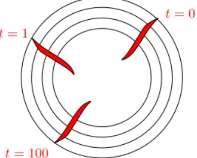
t= 100
t= 0 t= 1
Figure 3.2. An example of a system which is not mix- ing: for the harmonic oscillator (linearized pendulum) the angular velocity is independent of the action vari- able, so a disturbance in phase space keeps the same shape as time goes by.
The free transport equation can be solved explicitly: if fi is the datum at t= 0, then
(3.2) f(t, x, v) =fi(x−vt, v).
The simplicity of this formula is deceptive, and the free transport equa- tion displays much trickier behavior than one would imagine at first.
To study fine properties of this solution, it is most convenient to use the Fourier transform. Let us introduce the position-velocity Fourier transform
fe(k, η) = ZZ
f(x, v)e−2iπk·xe−2iπη·vdx dv,
where k ∈ Zd is dual to x ∈ Td, and η ∈ Rd is dual to v ∈ Rd. Then (3.2) implies
fe(t, k, η) = ZZ
fi(x−vt, v)e−2iπk·xe−2iπη·vdx dv (3.3)
= ZZ
fi(x, v)e−2iπk·(x+vt)e−2iπη·vdx dv (3.4)
=fei(k, η+kt).
(3.5)
This formula is similar to (3.2), up to swapping the two variables and changing the direction of time; in fact one may notice that the Fourier transform of the transport equation is a transport equation in Fourier
0. FREE TRANSPORT 31
space:
∂fe
∂t −k· ∇ηfe= 0.
Anyway, we deduce from (3.3) that
• f(t,e 0, η) = fei(0, η): the zero spatial mode of f is preserved;
• for fixed η and k 6= 0, fei(k, η + kt) −→ 0 as t → ∞, at a rate which is (a) determined by the smoothness of fi in v(Riemann–
Lebesgue lemma), (b) faster when k is large. In fact, the relevant time scale for the mode k is |k|t.
In particular, if fi is analytic in v then fei decays exponentially fast in η, so the mode k of the solution of the free transport equation will decay like O(e−2πλ|k|t). Also, if f is only assumed to be Sobolev regular, say Ws,1 in the velocity variable for some s > 0, then the Fourier transform will decay like O(|η|−s) at large values of |η|, so the mode of order k will decay like O((|k|t)−s).
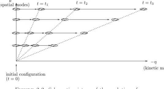
We can represent this behavior of the free transport equation, in Fourier space, as acascadefrom low to high velocity modes, the cascade being faster for higher spatial modes. Spatial oscillations generate, in large time, very strong kinetic oscillations.
k
(kinetic modes) initial configuration
(t= 0)
(spatial modes) t=t1 t=t2 t=t3
−η
Figure 3.3. Schematic picture of the evolution of en- ergy by free transport, or perturbation thereof; marks indicate localization of energy in phase space.
Remark3.1. In view of this discussion, the free transport equation appears to be a natural way to convert regularity into a time decay, which can in principle be measured from a physical experiment!
32 3. LINEARIZED VLASOV EQUATION NEAR HOMOGENEITY
Remark3.2. Even though the free transport equation is reversible, there is a definite behavior ast → ±∞: f(t, k, η) converges to 0 for alle k 6= 0, and tofei(0, η) fork = 0. This means that
f(t, x, v)−−−→weaklyt→∞ hfii, where the brackets stand for spatial average:
hhi(v) = Z
h(x, v)dx.
The convergence holds as long as the initial measure does have a den- sity, that is, fi is well-defined as an integrable function; and it is faster iffi is smooth. Note carefully that the convergence is weak, not strong;
in fact theL2norm off−hfidoes not converge to 0, it remainsconstant as t→ ∞. Indeed,
kf− hfik2L2 = ZZ
f2dx dv− Z
hfi2dv
is the difference of two quantities which are separately conserved.
Remark 3.3. Why don’t we see such phenomena as recurrence, which are associated with confined mechanical systems? The answer is that as soon as the distribution is spread out and has a density, we do not expect such phenomena because the system truly is infinite- dimensional. Recurrence would occur with a singular distribution func- tion, say Dirac masses, but we ruled out this situation. Of course one may argue that the true physical system is finite, however if the par- ticles are extremely numerous the recurrence times will be enormous, and the behavior is, hopefully, accurately described by the continuous model.
1. Linearization
Now let us go back to the Vlasov equation. Let f0 = f0(v) be a homogeneous equilibrium. We write f(t, x, v) = f0(v) +h(t, x, v), where khk ≪ 1 in some sense. Since f0 does not contribute to the force field, the nonlinear Vlasov equation becomes
∂h
∂t +v· ∇xh+F[h]· ∇v(f0+h) = 0, where
F[h](t, x) =− ZZ
∇W(x−y)h(t, y, w)dy dw =−∇xW ∗x,vh.
1. LINEARIZATION 33
When h is very small we expect the quadratic term F[h]· ∇vh to be negligible in front of the linear terms, and obtain
(3.6) ∂h
∂t +v· ∇xh+F[h]· ∇vf0 = 0.
The physical interpretation of (3.6) is not so obvious. Assume that we have two species of particles, one that has distribution h and the other one that has distribution f0, and that the h-particles act on the f0-particles by forcing, still they are unable to change the distribution f0 (like you are pushing a wall, to no effect). In this case, we can imagine that the changes in the f0 density would be compensated by the transmutation ofh-particles into f0-particles, or the reverse. Then the equation for f0 will be
(3.7) F[h]· ∇vf0 =S,
whereS is the source off0 particles, and thus the equation forhwould be
(3.8) ∂h
∂t +v· ∇xh=−S.
The combination of (3.7) and (3.8) implies (3.6). Thus, in some sense, equation (3.6) can be interpreted as expressing the reaction exerted by the “wall” f0 on the particle density.
We note that the last term on the right-hand side of (3.6) has the form F[h]· ∇vf0, where F[h] is a function of t and x, and f0(v) is a function of v. This property of separation of variables will be crucial.
As a start, it implies the statement below.
Proposition 3.4. If h = h(t, x, v) evolves according to the lin- earized Vlasov equation (3.6), then the function hhi = R
h(t, x, v)dx depends only on v and not on t.
An equivalent statement is that the linearized Vlasov equation has an infinite number of conservation laws: for any function ψ(v), R h ψ dv dx is a conserved quantity.
Proof of Proposition 3.4. First note thath∇xhi= 0 andhF[h]i= 0, since F[h] is a gradient. So (3.6) implies
∂thhi=−hv· ∇xhi −
F[h]· ∇vf0
=−v · ∇xhhi − hF[h]i · ∇vf0 = 0.
34 3. LINEARIZED VLASOV EQUATION NEAR HOMOGENEITY
2. Separation of modes
Let us now work on the linearized equation, in the form
(3.9) ∂h
∂t +v· ∇xh+F[h]· ∇vf0 = 0.
Solving this equation is a beautiful exercice in linear partial differential equations, involving three ingredients (whose order does not matter much): the method of characteristics, the integration in v, and the Fourier transform in x.
• First step: the method of characteristics. We apply the Duhamel principle to (3.9), treating it as a perturbation of free trans- port. It is easily checked that the solution of∂th+v· ∇xh=−S takes the form
h(t, x, v) =hi(x−vt, v)− Z t
0
S(τ, x−v(t−τ), v)dτ, where hi(x, v) =h(0, x, v).
• Second step: Fourier transform. Taking Fourier transform in both x and v yields
eh(t, k, η) = ZZ
hi(x−vt, v)e−2iπk·xe−2iπη·vdx dv (3.10)
−
ZZ Z t 0
S(τ, x−v(t−τ), v)e−2iπk·xe−2iπη·vdx dv dτ
= ZZ
hi(x, v)e−2iπk·(x+vt)e−2iπη·vdx dv (3.11)
− ZZZ
S(τ, x, v)e−2iπk·xe−2iπk·v(t−τ)e−2iπη·vdx dv dτ
=ehi(k, η+kt)− Z t
0
S τ, k, ηe +k(t−τ) dτ,
where I used the measure-preserving change of variables (x−vt, v)→ (x, v), and the obvious identityk·(vs) =v·(ks) to absorb the time-shift into a change of arguments in the Fourier variables.
3. MODE-BY-MODE STUDY 35
Now we note that the structure of separated variables in the term S and the properties of Fourier transform imply
S(τ, k, η) =e Fb(τ, k)·∇^vf0(η)
= (−∇W ∗ρ)b(τ, k)·∇^vf0(η)
= −2iπkWc(k)ρ(τ, k)b
· 2iπηfe0(η)
= 4π2k·ηWc(k)ρb1(τ, k)fe0(η), whereρ1(t, x) =R
h(t, x, v)dvis the first-order correction to the spatial density. Combining this with (3.10) we end up with
(3.12) eh(t, k, η) =ehi(k, η+kt)
−4π2Wc(k) Z t
0 ρb1(τ, k)fe0(η+k(t−τ))k·[η+k(t−τ)]dτ.
Third step: Integrate inv. This amounts to consider the Fourier mode η = 0 in (3.12):
b
ρ1(t, k) =ehi(k, kt)−4π2Wc(k) Z t
0 ρb1(τ, k)fe0(k(t−τ))|k|2(t−τ)dτ.
To recast it more synthetically:
(3.13) bρ1(t, k) =hei(k, kt) + Z t
0
K0(t−τ, k)ρb1(τ, k)dτ, where
(3.14) K0(t, k) =−4π2Wc(k)fe0(kt)|k|2t.
Now appreciate the sheer miracle: the Fourier modesρb1(k), k∈Z, evolve in time independently of each other! In a way this expresses a property of complete integrability, which can actually be made more formal.
Of course identity (3.14) is interesting only for k 6= 0; we already know that ρb1(t,0) =ehi(0,0) is preserved in time.
3. Mode-by-mode study
If k is given, equation (3.13) is a Volterra equation, which in principle can be solved by Laplace transform. Generally speaking, if we have an equation of the form ϕ =a+K∗ϕ, that is
ϕ(t) =a(t) + Z t
0
K(t−τ)ϕ(τ)dτ,
36 3. LINEARIZED VLASOV EQUATION NEAR HOMOGENEITY
then it can be changed, via the Laplace transform
(3.15) ϕL(λ) =
Z ∞ 0
e2πλtϕ(t)dt, into the simple equation
ϕL=aL+KLϕL, whence
(3.16) ϕL= aL
1−KL,
which is well-defined atλ∈RifAL(λ) andKL(λ) are well-defined (for instance if a and K decay exponentially fast and λ is small enough), and (careful!) if KL(λ)6= 1.
At this point it is useful to define the complex Laplace transform:
for ξ∈C,
(3.17) ϕL(ξ) =
Z ∞ 0
e2πξ∗tϕ(t)dt.
It is well-known that the reconstruction ofϕfrom its Laplace transform involves integratingϕL on a well-chosen contour in the complex plane, which has to go out of the real lineand should be chosen appropriately.
Since Landau, many authors have discussed this tricky issue, by now very classical in plasma physics.
However, the reconstruction gives more information than we need:
what we want is not the complete description of h, but its time- asymptotics. The following lemma will be enough to achieve this goal:
Lemma 3.5. Let K =K(t) be a kernel defined fort ≥0, such that (i) |K(t)| ≤C0e−2πλ0t;
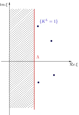
(ii) |KL(ξ)−1| ≥κ >0 for0≤ Re ξ ≤Λ.
Let further a =a(t) satisfy |a(t)| ≤α e−2πλt, and let ϕ solve the equa- tion ϕ =a+K∗ϕ. Then for any λ′ <min(λ, λ0,Λ),
|ϕ(t)| ≤C α e−2πλ′t, where C=C(λ, λ′,Λ, λ0, κ, C0).
Let us express this lemma in words: If the kernel K decays expo- nentially fast and satisfies the stability condition KL 6= 1 on a strip of width Λ>0 (see Fig. 3.4), then the solutionϕ decays in time at a rate which is limited only by the time-decay of the source, the time-decay of the kernel, and the width of the strip.