Automatic speech recognition: a survey
Mishaim Malik1 &Muhammad Kamran Malik2&Khawar Mehmood3&
Imran Makhdoom4
Received: 31 May 2020 / Revised: 4 September 2020 / Accepted: 13 October 2020
#Springer Science+Business Media, LLC, part of Springer Nature 2020
Abstract
Recently great strides have been made in the field of automatic speech recognition (ASR) by using various deep learning techniques. In this study, we present a thorough compar- ison between cutting-edged techniques currently being used in this area, with a special focus on the various deep learning methods. This study explores different feature extraction methods, state-of-the-art classification models, and vis-a-vis their impact on an ASR. As deep learning techniques are very data-dependent different speech datasets that are available online are also discussed in detail. In the end, the various online toolkits, resources, and language models that can be helpful in the formulation of an ASR are also proffered. In this study, we captured every aspect that can impact the performance of an ASR. Hence, we speculate that this work is a good starting point for academics interested in ASR research.
Keywords Speech recognition . ASR . Automatic speech recognition . Feature extraction . Classification models . Language models
* Mishaim Malik
[email protected] Muhammad Kamran Malik [email protected] Khawar Mehmood [email protected] Imran Makhdoom
1 Punjab University College of Information Technology (PUCIT), Lahore, Pakistan
2 Faculty of Punjab University College of Information Technology (PUCIT), Lahore, Pakistan
3 School of Engineering and Information Technology, University of New South Wales (UNSW) Canberra at ADFA, Canberra, Australia
4 Faculty of Engineering and IT, University of Technology Sydney, Ultimo, Australia Published online: 10 November 2020
1 Introduction
Speech is the most natural, efficient and preferred mode of communication between humans.
Therefore it can be assumed that people are more comfortable using speech as a mode of input for various machines rather than such other primitive modes of communication as keypads and keyboards. Automatic speech recognition (ASR) system helps us achieve this goal. Such a system allows a computer to take the audio file or direct speech from the microphone as an input and convert it into the text; preferably in the script of the spoken language. An ideal ASR should be able to “perceive” the given input, “recognize” the spoken words and then subsequently use the recognized words as an input to another machine so that some“action” can be performed on it [42,126,160]. Retrospectively, we consider ASRs to be the future means of communication between humans and machines.
Human speech and accents have huge variations, and this variation in speech patterns is one of the biggest obstacles in creating an autonomous speech recognition system. Bilingual or multilingual people tend to show more of these variations in their speech patterns than people who speak only one language. The same problem also arises when we add different factors such as gender, social style/dialect, speaking style and speed into the equation [40,112].
Another obstacle to creating an ASR is finding enough resources to train the ASR model.
Currently, such training models are available only for a handful of languages out of a total of approximately 6500 world languages.
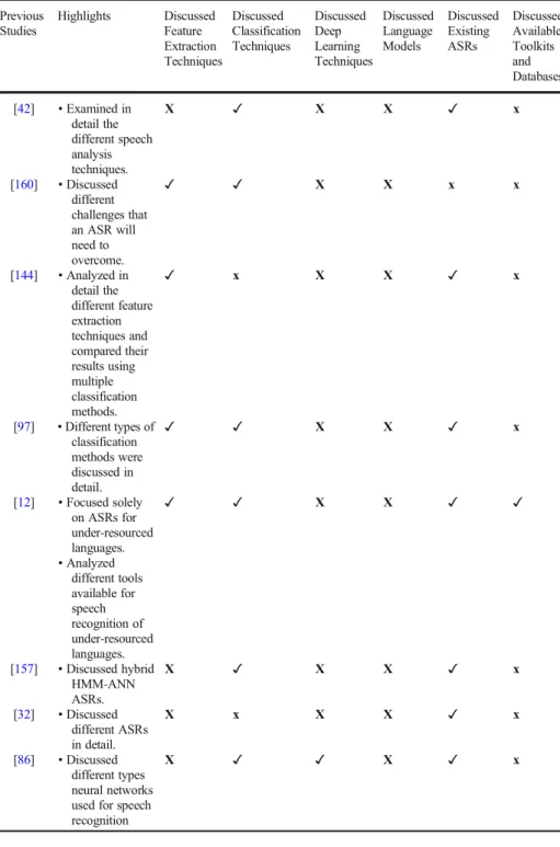
Over the past few years, many survey papers have been published to review and examine various aspects of ASR models presented over time. A recently published survey paper [160] discussed the challenges an ASR will have to overcome; and also discussed and analyzed the well-known models of ASR. It analyzes various challenges which include utterance approach and style, different speaker models, vocabulary size, and channel variability. The paper also highlighted three different classification ap- proaches; acoustic-phonetic approach, pattern recognition approach, and artificial intel- ligence approach. In another work [144], authors reviewed the efficiency of different feature extraction techniques including perceptual linear prediction (PLP), revised per- ceptual linear prediction (RPLP), and Bark frequency cepstral coefficients (BFCC). The paper compared the results of all these feature extraction techniques on different classi- fication models. [97] also presented some challenges to the real-world implementation of an optimal ASR system. The authors also classified ASR on the basis of speaker mode, speaking mode, and vocabulary size. The paper elaborates the front-end and back-end of an ASR system. The front-end of ASR consists of different feature extraction techniques in detail; whereas the back-end of ASR discussed various classification techniques extensively. Another survey paper [42], also reviewed different feature extraction tech- niques and classification models. In addition to that, the paper briefly defined different types of speech, speech analysis techniques and their impact on the performance of the system; and word error rate (WER), a metric used to calculate the accuracy of the results produced by an ASR. Similarly, [12] focused solely on ASR for under-resourced languages. This paper discussed the definition of under-resourced languages as well as why their preservation is important. The data collection methods of under-resourced languages and the basic structure of an ASR of under-resourced language were also discussed. Correspondingly, [157] comprehensively explained different hybrid HMM- ANN based ASRs, whereas, [32] gave an overview of different ASRs, as well as different approaches that can be used to recognize speech. This paper also briefly
discussed different types of speech recognition techniques. In another endeavor, [86] also discussed different types of ASRs, and neural networks based speech recognition approaches.
Table1presents the different highlights of the survey papers, which were discussed in the previous paragraph, in a compact and easily comprehensible form. The columns represent the different points that were covered or were missing in the discussed papers.
Most of the previously conducted studies failed to review the different feature extraction techniques and language models that play a vital part in the construction of an ASR. Similarly, the latest deep learning techniques were also not explained in the above-mentioned survey papers. Whereas, different online toolkits and databases that can help train an ASR were also missing from most of the studies. Hence, this study aims to evaluate the different feature extraction techniques and deep learning classification techniques. In addition to that, different online toolkits, databases, and language models were also assessed.
This study captures all the aspects of an ASR from the feature extraction phase to language models with the following objectives in mind:
& To understand and explain the basic structure of an ASR (shown in Fig.2) in detail, as well
as discuss how using different techniques at different stages can affect the overall performance of the system.
& Discuss in detail the different feature extraction and classification techniques being used
for the development of an ASR.
& Evaluate different toolkits and advancements made in language models and how they
affect the performance of an ASR.
& Encapsulate all of the information available regarding the different modules of an ASR,
including different state-of-the-art deep learning classification techniques.
The rest of the paper is organized as follows: Section2discusses different tools, resources and techniques that were used to perform this literature review. Section3presents a brief history of ASR, different techniques and datasets that can be employed to calculate the accuracy of the ASR, as well as the basic structure of an ASR. Section 4 explains the state-of-the-art techniques being used to extract features from an audio signal, whereas, Section5discusses techniques that can be used for classifying the extracted features. Section6explains language models, why they are needed, and their types. Section7presents the toolkits that can be used to perform different ASR related tasks, and finally, the survey is concluded in Section8.
2 Research methodology
Before researching this topic, a literature review is performed to determine the cutting edge technologies in this field. In this regard, IEEE,arxiv.org, Microsoft Academic, and Google Scholar were used to search and obtain the papers relevant to the research domain. Most of the relevant scientific seed words were first identified using the generic words and their synonyms related to the domain. Later on, specific seed words, which were identified from different publications, were used.
This method of searching ensured that all of the keywords were present in the titles of the research articles and publications. The AND operation was used to make sure all of the selected words were present in the titles. Double quotations were also used to ensure
Table 1 Highlights and shortcoming of the discussed surveys Previous
Studies
Highlights Discussed Feature Extraction Techniques
Discussed Classification Techniques
Discussed Deep Learning Techniques
Discussed Language Models
Discussed Existing ASRs
Discussed Available Toolkits and Databases [42] •Examined in
detail the different speech analysis techniques.
X ✓ X X ✓ x
[160] •Discussed different challenges that an ASR will need to overcome.
✓ ✓ X X x x
[144] •Analyzed in detail the different feature extraction techniques and compared their results using multiple classification methods.
✓ x X X ✓ x
[97] •Different types of classification methods were discussed in detail.
✓ ✓ X X ✓ x
[12] •Focused solely on ASRs for under-resourced languages.
•Analyzed different tools available for speech recognition of under-resourced languages.
✓ ✓ X X ✓ ✓
[157] •Discussed hybrid HMM-ANN ASRs.
X ✓ X X ✓ x
[32] •Discussed different ASRs in detail.
X x X X ✓ x
[86] •Discussed different types neural networks used for speech recognition
X ✓ ✓ X ✓ x
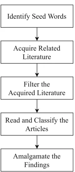
that all of the words were present together in titles i.e. present as a phrase rather than in the form of individual words. Out of all of the keywords that were used, “Speech Recognition” yielded the most but noisy results. Hence, to get better results, more queries were added to the seed words. The acquired articles were studied and state-of- the-art classification techniques, datasets, and feature extraction techniques were deter- mined. Fig.1presents an overview of the methodology followed to perform the research for this survey.
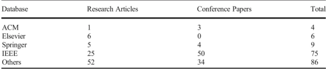
The three factors, that impacted how the literature was filtered, were relevance to the survey topic, how recently the research was conducted, and how thoroughly the paper covered the chosen topic. Table2shows the details of databases used to get the literature.
Identify Seed Words
Acquire Related Literature
Filter the
Acquired Literature
Read and Classify the Articles
Amalgamate the Findings
Fig. 1 Overview of search method
3 Background
Before we get into the technical details of the ASR systems, it is imperative to get familiar with the history of ASR. Hence, this section discusses the first speech recognition system followed by the advancements made to-date. This section also highlights different datasets that can be used for the training and testing purposes of an ASR as well as different evaluation techniques that can be used to measure the performance of an ASR.
Most of the speech recognition models are developed using a generic model. This generic model and its different types are also discussed in this section.
3.1 History and early developments
For quite some time computer scientists have been trying to create a machine that can talk and communicate like a human. Since the early 1950s, researchers have been trying to make a computer understand, interpret and reproduce human languages and speech [53]. The first speech recognition called Audrey was developed in the Bell Laboratories. This system could distinguish between different digits spoken by a single user [33]. Another system was developed in the MIT Lincoln Laboratories in 1959, which could distinguish between 10 phonemes for a single speaker [39]. In the 1970s a lot of important research was made in the area of speech recognition. Russian scientists developed a system that can be used to distinguish words [164]. The ideas of using dynamic programming [138] and pattern recog- nition algorithms [164] were also presented during these years. In the early 1980s, the hidden Markov model (HMM) was introduced. Even though the HMM was considered to be too simple to identify human languages [62], they still managed to replace the dynamic time warping technique that was being used [69]. In the later years of the 1980s, the n-gram model was introduced. In the early years of the 2000s, the HMM was being used in combination with a feed-forward artificial neural network (ANN) [14]. Nowadays, long-short term memory (LSTM) [14], a type of recurrent neural network (RNN), is being used for speech recognition in combination with different deep learning techniques.
3.2 Evaluation techniques
Evaluation is one of the most important aspects of a conducted research because of its importance this section explains in detail different metrics that can be used to evaluate the performance of an ASR. The performance of a speech recognition system usually depends on two factors, the accuracy of the output produced as well as the processing speed of the ASR.
Table 2 Databases used for acquiring literature
Database Research Articles Conference Papers Total
ACM 1 3 4
Elsevier 6 0 6
Springer 5 4 9
IEEE 25 50 75
Others 52 34 86
3.2.1 Speed
The following method can be used to calculate the processing speed of an ASR:
3.2.2 Real-time factor
The real-time factor (RTF) is the most commonly used metric for calculating the speed of a proposed model. The RTF can be computed by using the following formula:
RTF¼P I
where P is the time taken by the system to process the input and I is the duration of the input audio. If RTF equals 1, then the input audio was processed in“Real-Time”. RTF is a highly hardware-dependent value and it is not only limited to calculating the speed of a speech recognition model. It can be used to calculate the speed of any model that can process an audio or video input.
3.2.3 Accuracy
The following methods can be used to measure the accuracy of an ASR:
Word error rate The accuracy of an ASR is hard to calculate as the output produced by the ASR may not have the same length as the ground truth. Word error rate (WER) is the commonly used metric to estimate the performance of an ASR, as it calculates error on word level rather than phoneme level [124]. The WER can be calculated using the following formula:
WER¼SþDþI N
Where S is the number of substitutions performed in the output text as compared to the ground truth. D is the number of deletions performed, and I is the number of insertions performed. N is the total number of words in the ground truth.
Word recognition rate Word Recognition Rate (WRR) is a variation of WER that can also be used to evaluate the performance of an ASR. It can be calculated using the following formula:
WRR¼1−WER
¼N−S−D−I N
¼H−I N
Where H = N - (S + D) represents the total number of correctly guessed words.
3.3 Datasets
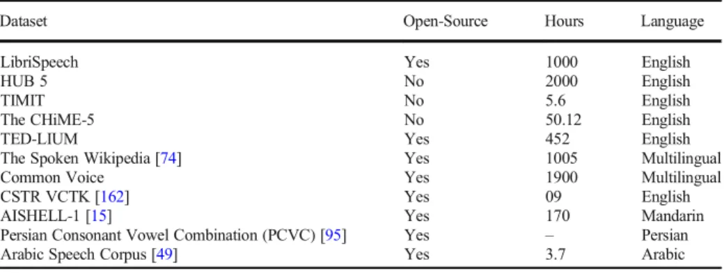
A dataset is essential for the training and testing of an ASR. This section discusses in detail some of the commonly used open-source as well as paid datasets. Table3provides a list of the available speech datasets; and their salient features such as total time and spoken languages.
3.3.1 LibriSpeech
LibriSpeech [116] is one of the most frequently used open-source speech-to-text corpus. This dataset consists of 1000 h of audiobooks along with their transcriptions. Because of the large magnitude of the collected data, it was divided into three sets. The first set is comprised of 100 h of training data, the second contains 360 h of training data, and the last set has 500 h of training data. The development set and the testing set have 10.8 and 10.1 h’worth of data, respectively.
3.3.2 2000 HUB5 English evaluation transcripts
2000 HUB5 English evaluation transcripts is the dataset used in deep speech model [50]. It consists of 2000 h of conversational audio and their corresponding transcriptions. This dataset consists of forty source files, all with their corresponding text. Twenty of these files were scripted; a robot operator announces the topic of conversation before the conversation starts.
The rest of the twenty files consist of unscripted conversations between Native English Speakers.
3.3.3 TIMIT acoustic-phonetic continuous speech Corpus
Another commonly used dataset for speech recognition is the TIMIT acoustic-phonetic continuous speech corpus [45]. This dataset consists of the recordings of 6300 phonetically rich sentences, read by 630 speakers, where 30% of them are female, and the rest are male speakers. The training set consists of 3.14 h of recording; the rest is divided into the test and development set respectively.
Table 3 List of speech datasets that can be used for training an ASR
Dataset Open-Source Hours Language
LibriSpeech Yes 1000 English
HUB 5 No 2000 English
TIMIT No 5.6 English
The CHiME-5 No 50.12 English
TED-LIUM Yes 452 English
The Spoken Wikipedia [74] Yes 1005 Multilingual
Common Voice Yes 1900 Multilingual
CSTR VCTK [162] Yes 09 English
AISHELL-1 [15] Yes 170 Mandarin
Persian Consonant Vowel Combination (PCVC) [95] Yes – Persian
Arabic Speech Corpus [49] Yes 3.7 Arabic
3.3.4 CHiME-5
The CHiME-5 [8] is another dataset that can be used for training an ASR. The main idea behind this dataset was to aid in the creation of a genuinely robust speech recognition system. This dataset contains 50.12 h of recorded conversations in real home environments. The training set of the dataset consists of 40.33 h of data with almost 80,000 utterances. The development set has 4.27 h’worth of data with a little over 7000 utterances. Lastly, the testing set 5.12 h of data with 11,000 utterances.
3.3.5 TED-LIUM Corpus
The TED-LIUM Corpus [131] is an open-source speech dataset containing 452 h of ted talks and their corresponding transcriptions.
3.3.6 Common voice
Common Voice is a great project started by Mozilla, to gather speech data. It is an open-source project, where people can donate their voices, to read out a given sentence, or their time, that will be required to validate whether a particular audio file matches its corresponding tran- scription. They have gathered 2400 h of data of different languages, out of which 1900 h of data is validated. Currently, they can provide speech datasets of English, German, French, Welsh, Turkish, and 13 other languages.
3.3.7 The spoken Wikipedia
This free dataset contains 1005 h’worth of audio files of three different languages English, German, and Dutch. The English dataset is the largest consisting of 1339 pages of Wikipedia spoken by 465 speakers. This portion of the dataset consists of 395 h of audio files. The German dataset consists of 386 h of audio files covering the content of 1014 pages spoken by 350 speakers. The Dutch dataset is quite small as compared to the other two languages; it consists of only 224 h of data even though it covers the most number of pages of 3171 spoken by 145 speakers.
3.3.8 CSTR VCTK Corpus
This dataset consists of 400 sentences spoken by 109 distinct speakers. All of the speakers are native English speakers with varying ages, gender, and accents. This dataset contains almost 9 h of audio data.
3.3.9 AISHELL-1
This open-source dataset offers 170 h of Mandarin speech data. The dataset consists of 400 unique speakers of all genders and ages. To make the dataset more robust speech on different subjects such as Finance, Science and Technology, Entertainment and Sports were used.
3.4 The architecture of an ASR
The function of an ASR is to take input of a sound wave and convert the spoken speech into text form; the input could be either taken directly using a microphone or as an audio file. This
problem can be explained in the following way: for a given sequence input sequence X, where X = X1, X2,…., Xn, where n is the length of the input sequence, the function of an ASR is to find a corresponding output sequence Y, where Y = Y1, Y2,…., Ym, where m is the length of the output sequence. And the output sequence Y has the highest posterior probability P(Y|X), where P(Y|X) can be calculated using the given formula:
W¼argmax P Wð =XÞ
¼argmax P Wð ÞP Xð =WÞ P Xð Þ
where P(W) is the probability of the occurrence of the word, P(X) is the probability that X is present in the signal, and P(X|W) is the probability of the acoustic signal W occurring in correspondence to the word X.
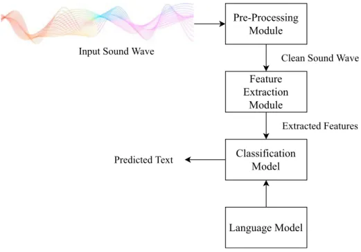
An ASR can generally be divided into 4 modules: a pre-processing module, a feature extraction module, a classification model, and a language model, as shown in Fig.2. Usually the input given to an ASR is captured using a microphone. This implies that noise may also be carried alongside the audio. The goal of preprocessing the audio is to reduce the signal-to-noise ratio [176]. There are different filters and methods that can be applied to a sound signal to reduce the associated noise. Framing, normalization, end-point detection and pre-emphasis are some of the frequently used methods to reduce noise in a signal [105, 114, 135]. Pre- processing methods also vary based on the algorithm being used for feature extraction. Certain feature extraction algorithms require a specific type of pre-processing method to be applied to its input signal.
After pre-processing, the clean speech signal is then passed through the feature extraction module. The performance and efficiency of the classification module are highly dependent upon the extracted features [3, 78,178]. There are different methods
Input Sound Wave
Pre-Processing Module
Feature Extraction
Module
Classification Model
Language Model
Clean Sound Wave
Extracted Features
Predicted Text
Fig. 2 Basic structure of an ASR
of extracting features from speech signals. Features are usually the predefined number of coefficients or values that are obtained by applying various methods on the input speech signal. The feature extraction module should be robust to different factors, such as noise and echo effect. Most commonly used feature extraction methods are Mel- frequency cepstral coefficients (MFCCs), linear predictive coding (LPC), and discrete wavelet transform (DWT) [40,78,112,127].
The third and final module is the classification model; this model is used to predict the text corresponding to the input speech signal. The classification models take input of the features extracted from the previous stage to predict the text. Like the feature extraction module, there are different types of approaches that can be applied to perform the task of speech recognition. The first type of approach uses joint probability distribution formed using the training dataset, and that joint probability distribution is used to predict the future output. This approach is called a generative approach; HMM and Gaussian mixture models (GMM) are the most commonly used models based on this approach. The second approach calculates a parametric model using a training set of input vectors and their corresponding output vectors. This approach is called the discriminative approach; Support Vector Machines (SVM) and ANN are its most common examples [11, 87]. Hybrid approaches can also be used for classification purposes; one example of such a hybrid model is that of a HMM and ANN [151].
The language model is the last module of the ASR; it consists of various types of rules and semantics of a language. Language models are necessary for recognizing the phoneme predicted by the classifier; and is also used to form trigrams, words or sentences using all of the predicted phonemes of a given input. Most modern ASRs are designed to work without Language Models as well. Such ASRs can predict words and sentences spoken in the given input, but their efficiency can be increased signif- icantly by using a language model [18].
3.4.1 Types of ASR
As shown in Fig.3, an ASR can be classified on the basis of speaker models, vocabulary being used, channel variability, and speaking style, which can be further classified into two types, utterance speed, and utterance approach.
& Speaker Mode
The purpose of creating an ASR is that it can transliterate any language for any speaker.
Languages differ in terms of phonetics, character set, and grammar rules; speakers vary in terms of voice pitch, accent, and personality. Every speaker has a unique voice and speaking style; on this basis, an ASR can be classified into the following three types:
4 Speaker-independent models
Speaker-independent ASRs are developed to recognize multiple speakers. Such systems are not trained for a particular user and are one of the most complex types of systems to design.
These systems might offer less accuracy than other methods but are more flexible and can have wide usage in the real world.
5 Speaker-dependent models
Speaker-dependent ASRs are developed to recognize a single user or multiple pre-trained users. Such systems are easily trained and also offer better accuracy than speaker-independent ASRs. But they will not be able to produce the same level of accurate results for voices outside of the user pool that they were trained on.
6 Speaker adaptive models
Speaker adaptive ASRs lie somewhat in between speaker-independent and speaker-dependent ASRs. These systems are trained in such a way that they can learn new speech patterns whenever a new speaker presents itself.
& Vocabulary Size
The vocabulary of an ASR matters a lot as it can affect the complexity, processing time, and the accuracy of the system. The larger the size of the vocabulary, the more complex the system will be; more time will also be required to train the system. The accuracy of the system will also reduce because of the more similar sounding words in the vocabulary. Some ASRs might
ASR
Speaker Mode
Speaker Independent
Vocabulary Size Speaking Style Channel Variability
Speaker Dependent
Speaker Adaptive
Small
Medium
Large
Very Large
Utterance Approach
Isolated Words
Connected Words
Utterance Style
Continuous Speech
Spontaneous Speech Out of
Vocabulary
Fig. 3 Types of ASR
require a vocabulary of tens of words, for example, a number speech recognition system or a character recognition system. While for others even tens of thousands of words may not be enough; for example, for an ASR that recognizes the English language will require a larger vocabulary than a number recognizing ASR.
7 Small
A small vocabulary can consist of tens of words.
8 Medium
A vocabulary containing hundreds of words is considered to be a medium-sized vocabulary.
9 Large
A large vocabulary can consist of thousands of words.
10 Very large
A very large vocabulary usually has tens of thousands of words.
11 Out of vocabulary
All the words that are not part of vocabulary are mapped as unknown words.
& Speaking Style
In terms of speech recognition, an utterance is a spoken word. A single word, few words, a single sentence, and few sentences can be considered as an utterance as well. Based on utterances type, multiple approaches can be used to develop an ASR.
12 Utterance approach
An utterance is divided into two types: isolated and connected words.
a Isolated Words
A system that is based on the isolated word type of utterance requires its users to take a well- defined pause between each spoken word. This does not necessarily mean that the system will only take one-word input at a time and produce one-word output. Such systems can take multiple words as input but will only process one of them at a time.
b Connected Words
Connected words, on the other hand, consists of a system that works with connected utterances and will take a nominal or no pause between two or more words. Such systems can take an input of multiple words at a time and process them as a whole rather than individually.
13 Utterance style
Since most people have their speaking style, utterances can also be divided into two types on this basis. These two types are continuous and spontaneous speech [82].
a Continuous Speech
In continuous speech utterances, the users of the system are allowed to speak almost naturally.
These types of utterances do not require a pause between words. The input given to the system is considered as a whole and is not divided into individual words based on pauses.
b Spontaneous Speech
Spontaneous speech utterances are completely natural. Such utterances may include bogus starts, coughing, laughter, and words like“um”and“ah”, etc. These systems are very difficult to develop as the system will require a very large vocabulary. It will also need to be able to differentiate between valid words and other sounds.
& Channel Variability
Another way of classifying ASRs is based on the quality of the input channel. Some ASRs require input signals that are recorded in a clean environment i.e. without any background noise. Noise is unnecessary or unwanted information in the input speech signal. It can be anything from the chirping of birds in the background to distortion from the sound not being recorded correctly. Sometimes the input sound wave also gets distorted when we change its channel by using different software.
Besides noise, the difference in ages, gender, accent, environment, and speaking speed are also considered as variations in the input signal. An ASR should be able to cope with all of the different types of background noises or variations in the input speech signal [40,71].
14 Feature extraction
The process of feature extraction is applied to remove irrelevant information from the signal. A good feature extraction algorithm should be able to extract the features in real-time and should contain maximum information. Feature extraction algorithms can also be classified based on speech features: temporal and spectral features. The temporal analysis techniques analyze the audio signal in its original form, the time domain. In spectral analysis, as the name implies, the spectral representation of the speech signal is used, the frequency domain. Some of the
methods used for feature extraction are the MFCC, PLP, DWT, relative spectral-perceptual linear prediction (RASTA-PLP), and LPC.
14.1 Spectral feature analysis
14.1.1 Mel-frequency Cepstral coefficients
MFCC [37,114] is one of the most powerful and most commonly used technique for feature extraction [22,27,76,98,111,156].
A human ear does not perceive the voice or pitch of a sound linearly. Since many of the applications do not work well with the change in frequency, a scale was introduced in the 1940s, called the Mel-scale. The Mel-scale was developed when researchers were experimenting with how a human ear perceives pitch. It linearized the human auditory system to a linear scale [156]. The experimentations that were performed to develop this scale concluded that only the frequencies between 0 to 1000 Hz could be linearized to the Mel- scale. The values that do not fall in this range were considered to be logarithmic [147]. The following formula can be used to linearize a frequency to Mel-scale:
Fmel¼ 1000
log 2ð Þ 1þ FHz
1000
Here Fmel is the resultant linearized frequency, and FHz is the original frequency of the function.
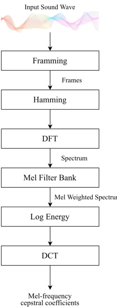
As we know, a continuous audio function has different values at different points of time. To simplify processing, the audio signal is divided into small frames of either 25 ms [22,111, 156] [35,137,155] or 30 ms [54,147], where 10 ms of continuous frames overlap. Once the audio signal is divided into frames, each frame is multiplied with the hamming window function, and discrete Fourier transform (DFT) is applied to the result [105]. Sometimes fast Fourier transform (FFT) is also applied to reduce the processing time of the overall process [114]. The results of the Fourier transform is then used to calculate filter bank and then the filter bank is used to calculate log energy outputs using the given below formula:
Xi¼log10 N−1∑
k¼0jX kð Þj Hið Þk
; for i¼1;…;M
WhereHi(k) is the filter bank, X(k) is the k-th window of source signal X, M is the length of the Fourier Transform, and Xiis the log energy outputs. In the end, Discrete Cosine Transform (DCT) is applied on the log energy outputs using the formula given below:
Cj¼ ∑M
i¼1Xicos j i−1 2
π M
; for j¼0;…::;J−1
Where Cjis the mel-frequency cepstral coefficients, j is the serial index, and J is the total number of MFCC features. DCT allows most of the energy to be preserved while achieving dimensionality reduction by discarding coefficients with high values but low energy [105, 147]. A block diagram that summarizes the process of MFCC is illustrated in Fig.4.
Though the frames of an input sound are divided into either frame of 25 ms or 30 ms, the influence of one phoneme can extend over more than one frame. Thus, the timing correlation between multiple frames should also be considered for more accurate results. It can be taken
under consideration by using the delta and delta-delta features of MFCC; the delta MFCC has the addition of the dynamic features; whereas the delta-delta MFCC includes the acceleration features. So, the feature vector obtained from the MFCC algorithm contains three types of features. The first type is the static features, the second is the difference between static features of successive frames or delta features, and the third is the difference between successive dynamic features or delta-delta features. An MFCC feature vector usually consists of thirty- nine dimensions; thirteen for each type of feature; static, dynamic (delta), and acceleration (delta-delta). Another variation of the MFCC feature vector contains the normalized log energy
Input Sound Wave
Framming
Hamming
DFT
Mel Filter Bank
Log Energy
DCT
Spectrum Frames
Mel Weighted Spectrum
Mel-frequency cepstral coefficients
Fig. 4 Block diagram of MFCC process
as well; this feature vector also has thirty-nine dimensions, the static feature vector has twelve dimensions in this type instead of the usual thirteen [30,35,98,156].
MFCC may be the most commonly used feature extraction method, but it’s not without its limitations. One of the negative features of this algorithm is that it’s not adaptive to noise. If even one of the frequency bands in the input signal is distorted the results of MFCC will suffer greatly [47,63,91,106,111]. Another negative feature is the assumption made during the process of framing; that one phoneme can be mapped to the audio of 25 to 30 ms. As we all know, different speaking styles and accents can sometimes drag one phoneme over the space of two or constrict the information of two phonemes into one frame, so this assumption may not yield the best results. Mean and variance normalization (MVN) [63], cepstral mean normalization [91,111], and histogram equalization [63] are some of the techniques that can be used to make MFCC more robust.
14.1.2 Linear predictive coding
Linear predictive coding (LPC) [37,114], released in 1984 [113], is one of the most powerful methods of extracting features from a speech signal, and hence has become one of the most commonly used feature extraction algorithm [107, 108,151, 174]. Unlike MFCC, which resembles the human auditory system, LPC imitates the basic structure of the vocal tract [30].
It can also be easily compared with the basic model of speech production which is also modelled as a linear but time-varying system for both periodic pulses or voiced sounds and random noises [48,135,157].
The basic idea behind this algorithm is that the current sample can be represented as a linear combination of all of the previous samples. The LPC analysis can be calculated by first dividing the input audio into frames and then performing the process of windowing on these frames to make sure there are no discontinuities in the beginning or end of any frame. The last step of the process is to calculate the auto-correlation between the frames. And then the LPC analysis is performed on the obtained auto-correlation values, by using Durbin’s Method [48, 108,113] or by using the formula given below [48,178]:
s n½ ≈ ∑p
k¼1
a k½ s n−k½
Where s[n] is the current sample point, p is the total number of previous sample points, which are also called predictors [4], and a[k] which is the predictor coefficient.
The main goal of LPC is to calculate the coefficients of a[k] for each frame where E, the total squared prediction error, is minimum. So, once the LPC analysis is performed, the total squared prediction error can be calculated using the formula given below:
E¼∑
n
s n½ − ∑p
k¼1a k½ s n−k½ 2
14.1.3 Linear predictive Cepstral coefficients
After performing an LPC analysis on the given input audio, the following formula is applied to get linear predictive cepstral coefficients (LPCC) [125]:
bv n½ ¼lnð Þ;p for n¼0 bv n½ ¼a n½ þn∑−1
k¼1
k
n bv k½ a n−k½ ; for1≤n≤p
Where p is the total number of sample points,bv n½ are cepestral coefficients, and n is the number of samples present in the anaysis frame.
Recent research [21] examined the performance of LPCC as compared to MFCC. The system that was used to study these feature extraction algorithms could identify twelve Hindi words spoken by five different speakers. This system showed that LPCC and MFCC had similar results. Another research [165] showed that LPCC was 10% more efficient and 5.5%
faster than MFCC. Fig.5sums up the process of LPCC in the form of a block diagram.
14.1.4 Perceptual linear prediction
PLP uses transformations that are based on a human auditory system. This algorithm has three main characteristics; the spectral resolution of the critical band, application of intensity-loudness power law, and equal loudness curve reduction. By remapping the frequency axis to the Bark scale, PLP incorporates critical band spectral resolu- tion into its spectrum estimate and produces a critical band spectrum approximation.
This approximation integrates the energy in critical bands. As we know, human hearing is more sensitive to the middle-frequency range of audible spectrum at conversational speech levels. PLP incorporates this phenomenon in the algorithm by multiplying the loudness curve with the critical spectrum band. By doing this, the high and low-frequency regions are suppressed between the range of 400 kHz and 1200 kHz, which is the mid-range. A nonlinear relationship exists between the perceived loudness and the intensity of sound. Cube root amplitude compression of the loudness equalized critical band spectrum estimate is used to approximate the power law of hearing [88].
To calculate the coefficients of PLP, windowing is performed on the input signal, and then an FFT is applied on the windowed input signal. The resultant signal is then converted into Bark Scale using the formula given below:
θð Þ ¼Bi 2:5∑
B¼−1:3
X Bð −BiÞ j j2ψð ÞB
Input Sound Wave
Framming Windowing
Auto-correlation LPC Analysis
Frames
Cepstral Analysis
LPCC Fig. 5 Block diagram of LPCC
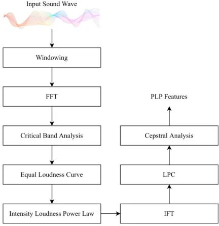
Where is the Bark-scaled frequency, and X is the input signal. The Bark scaled frequency ensures that the critical band frequency selectivity is modelled inside the range of human cochlea [105,125]. Once the Bark-scaled frequency is calculated, it is weighted according to the equal-loudness curve, and then the intensity-loudness power law is applied to the acquired weighted frequency. Inverse Fourier transform (IFT), linear predictive analysis, and cepstral analysis are performed in order to get the PLP coefficients [105,125]. Fig.6summarizes the steps performed in PLP in the form of a block diagram.
The research performed in [55] showed an HMM-ANN system that recognized English language phonemes and used PLP as its feature extraction algorithm. The system used TIMIT corpus for training and testing purposes. The accuracy achieved was 64.9%, but when the system was tested on HTIMIT, which consists of speech data collected over different telephone channels, the accuracy dropped to 34.4%. The research performed in [44] discussed the performance of PLP in comparison with MFCC in noisy environments. The research used two different types of noise signals:
white and street noise. The system used was a multi-lingual system that could recog- nize words of six languages: Hungarian, English, French, Italian, Spanish, and German.
The results obtained from the research showed that PLP achieved 0.2% more accuracy than MFCC.
Input Sound Wave
Windowing
FFT
Critical Band Analysis
Equal Loudness Curve
Intensity Loudness Power Law IFT
LPC Cepstral Analysis
PLP Features
Fig. 6 Block diagram of PLP analysis
14.2 Temporal feature analysis
14.2.1 Relative spectra–perceptual linear prediction
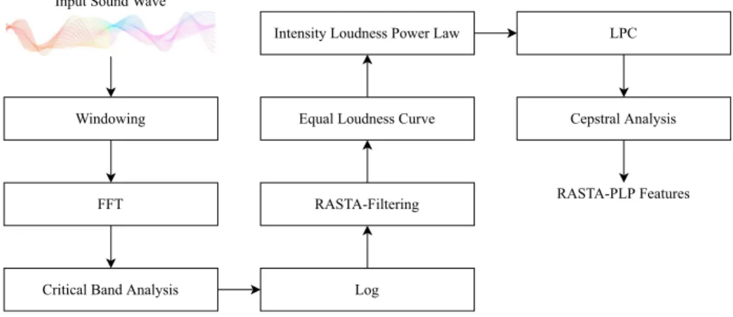
RASTA-PLP analysis specializes in noisy environments by merging RASTA and PLP analysis. It can easily be observed that often training and testing data’s conditions differ, testing data usually contains more real-life factors such as noise, inter-speaker variations, intra- speaker variations, and a difference in the transmission channel. The basis of RASTA [139]
analysis is that the temporal properties of the environment, in which the input signal was recorded, varies from the temporal properties of the speech. So, by using a band-pass filter on all frequencies in each sub-band, the short-term noise is smoothed, and the difference in training and testing environments is reduced significantly. The block diagram shown in Fig.7 explains the steps performed to calculate RAST-PLP features.
Another research [56], compared LPC, MFCC, and RASTA-PLP as feature extraction techniques for a system that recognized digits of Kannada language. The input signals were pre-processed using wavelet transforms; DWT was used for clean signals, whereas, the wavelet packet transform (WPT), was used for noisy signals. For clean speech signals, MFCC had the highest accuracy of 94%, followed by LPC, which had an accuracy of 82%, and RASTA-PLP had an accuracy of 54%. For the noisy signals without pre-processing, RASTA- PLP had the highest accuracy of 73%, followed by MFCC, with an accuracy of 60%, and LPC had the lowest accuracy of 53%. After applying the WPT, the accuracies of all three feature extraction methods were increased, with RASTA-PLP having the highest accuracy of 83%.
Hence we can easily say that, for noisy datasets, RASTA-PLP performs much better than any other feature extraction method, whereas it may not perform as well for clean speech signals. It was also observed in [56] that RASTA-PLP can have an even better performance when combined with WPT.
14.2.2 Discrete wavelet transform
We know that speech signals are not stationary and contain both temporal and frequency information. Even though most algorithms focus only on frequency information, temporal information is equally important [5,121,137]. DWT takes into consideration the temporal
Input Sound Wave
Windowing
FFT
Critical Band Analysis Log
RASTA-Filtering Equal Loudness Curve
Intensity Loudness Power Law LPC
Cepstral Analysis
RASTA-PLP Features
Fig. 7 Block diagram of the process of RASTA-PLP
information present in the input audio signal by re-scaling, shifting, and then analyzing the mother wavelet to obtain the temporal information present in the input signal. Because of this, the input signal is not only analyzed on different frequency levels but with different resolutions as well [5,121].
So, DWT is based on multi-resolution analysis, according to which lower frequency components appear for a much longer duration than the higher frequency components in a speech signal. Because of this reason, instead of using the same size window, different sizes of windows are used for lower and higher frequency components. For a higher frequency component, a narrow window is used, and a wider one is used for lower frequency components [121]. DWT was created to replicate the working of a human auditory system, where decreasing frequency resolution is used to analyze the increasing frequencies present in a signal [135].
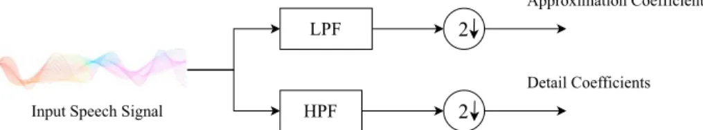
The DWT analysis divides the input speech signal into two types of coefficients: detail and approximation coefficients. The detail coefficients represent the low-scale high-frequency components of the input signal, and approximation coefficients represent the highscale low- frequency components [78, 127]. DWT can be performed using a formula proposed by Stephane G. Mallat [96] this is a fast pyramidal algorithm that uses multi-rate filter-banks, called Mallattree decomposition. The algorithm decomposes the signal into detail and approx- imation coefficients, as shown in Fig.8.
The input speech signal is passed through a high-pass and a low-pass filter to get the detail and approximation coefficients, and then the results obtained from filters are down-sampled by two, the results obtained after down-sampling are the required coefficients. The process of applying the filters and down-sampling can be mathematically expressed in the form of the formulas given below [5]:
ylow½ ¼k ∑
n
x n½ h½2k−n yhigh½ ¼k ∑
n
x n½ g½2k−n
Where x[n] is the input signal, h[n] is the low-pass filter, and g[n] is the high-pass filter. The approximation coefficients can be further divided by using the same steps repeatedly.
Speech signal often lies in the lower frequency components of a signal, even if the higher frequency components are removed from a signal, the speech present in the signal will still be understandable even though the overall sound of the signal will be different. The research done in [43] shows that instead of using the detail coefficients, using approximation coefficients to generate octave achieves better accuracy.
DWT coefficients are obtained by concatenating the approximation and detail coefficients starting from the last decomposition level. The total number of decomposition levels is chosen based on the frame size. The frame sizes between 3 and 6 octaves are commonly used. The filters used for computing DWT should be a quadrature mirror filter (QMF), which can be calculated using the formula given below:
Input Speech Signal
LPF
HPF
2
2
Approximation Coefficients
Detail Coefficients
Fig. 8 Decomposition of speech signal into high frequency and low-frequency components
g L−1−n½ ¼ð Þ−1 nh n½
where L is the length of the filter. The QMF relationship will ensure that the original input can be perfectly reconstructed from the decomposed signal.
DWT is very robust to noise as it works with localized time and frequency information.
Hence, if one of the frequency bands of the input signal is altered by the noise, it will not affect all of the coefficients produced by this algorithm. Due to this reason, many of the researches related to ASRs used DWT as their feature extraction method [43,64,100,151,167].
14.2.3 Wavelet packet transform
WPT is very similar to DWT. The only difference is that the detail and approximation coefficients are more decomposed in WPT as compared to DWT [78]. The research done in [105] compared the performance of DFT based algorithms with algorithms based on DWPT for the task of speech recognition. One of the DFT based algorithm under consideration was MFCC. This research showed that DWPT based methods performed better as compared to DFT based algorithms. When compared against MFCC, a reduction of 20% in word error rate was achieved with a DWPT based method. Another research [105], compared the perfor- mances of WPT against DWT. The system being used was an ASR that could identify the Malayalam language. Here DWT outperformed WPT, as DWT achieved an accuracy of 89%, as compared to, WPT which could only achieve 61%.
14.3 Summary
From the above discussion, it was easy to conclude that in the past, feature extraction techniques that focused on spectral analysis preferred over techniques that used temporal analysis. However, over the past few years, it became obvious that spectral analysis alone was not enough to gather maximum information from the input speech signal. Hence, the wavelet techniques, which used temporal analysis, were used in some researches instead of MFCC and LPC. DWT achieved better results for the task of phoneme recognition than the more commonly used MFCC.
Storage space is a factor that should be taken into consideration when discussing feature extraction techniques. DWT is preferred if there is limited space available, as its feature vector is much smaller in size. There are other feature extraction techniques, such as Principal Compo- nent Analysis (PCA), Vector Quantization (VQ) and Linear Descriptive Analysis (LDA), that can also be used in combination with other methods, such as MFCC, to reduce the dimensions of their feature vectors. Different researches used VQ with MFCC [153] and DWT [127] to utilize its clustering property to improve the performance of their ASR. Whereas the PCA and LDA were used to reduce the dimensionality of the feature vector, all the while making the system more robust [38,60,163]. Another point to be considered when selecting a feature extraction technique is the type of environment the ASR will be deployed in. In clean environments, MFCC, PLP, and LPC achieved good accuracies; whereas, for noisy environ- ments, DWT, LPCC, and WPT showed better results. One way to make an ASR more robust is to combine the MFCC, PLP, and LPC with either DWT or WPT. Another way is to use RASTA-PLP, which performs best in a noisy environment but not in clean environments.
Table 4 summarizes the advantages and disadvantages of all of the above-mentioned techniques.
15 Classification
After features are extracted, they are passed as input to a classifier. This is one of the most important and time-consuming modules, as a classifier predicts the phoneme or word that is spoken in the input signal. The job of a classifier is to learn the relationship between the given input audio features, and their corresponding text or phonemes. They are first trained using the training data, which should be big enough for a classifier to recognize the specific patterns
Table 4 Advantages and disadvantages of the discussed feature extraction methods Feature Extraction
Method
Advantages Disadvantages
Mel-Frequency Cepstral Coefficients [84]
•MFCC provides good discrimination between phonemes [48].
•It closely resembles the human auditory perception system because it is not linear [48].
•It can capture important information present in the signal [48].
•It is not robust to noise [76] [111].
•It may not be able to map continuous phonemes correctly.
Linear Predictive Coding [91]
•It represents the vocal tract and is an accurate and reliable method of getting features [103].
•It is very robust and can extract features even from speech signals that have a low bit rate.
•It can not successfully distinguish between words containing similar-sounding phonemes [142].
•It might not be able to represent speech, as LPC assumes that the given signal is stationary and hence, cannot analyze local events accurately.
•The feature coefficients have a high correlation among them.
Linear Predictive Cepstral Coefficients [109]
•The high correlation of LPC is removed by applying the cepstral analysis [119].
•It is more robust than a simple LPC analysis.
•It might not be able to represent speech properly, as it assumes that the given signal is stationary and cannot analyze local events accurately.
•It cannot retain prior information in the testing phase.
Perceptual Linear Prediction [88]
•The difference between voiced and unvoiced inputs is reduced.
•It is independent of the length of the vocal tract.
•The feature vector produced has relatively fewer dimensions.
•The feature vector being produced is highly dependent on the spectral balance of the formant amplitudes.
•Channel, noise, and the equipment used to get the input signal can easily change the spectral balance.
Relative Spectra–Perceptual
Linear Prediction [72]
•It is very robust.
•It removes slow and fast variations present in the speech signal [57].
•RASTA-PLP captures low modulation frequencies, which correspond to speech in a signal [20].
•It doesn’t perform well for speech signals without noise.
Discrete Wavelet Transform [168]
•DWT considers temporal information present in the signal alongside frequency information.
•It can perform de-noising tasks successfully [99].
•The input signal can be recreated perfectly from the decomposed parts.
•The same base wavelet is used for all input signals, which makes this algorithm inflexible.
Wavelet Packet Transform [120]
•Same as DWT, the only difference is that this algorithm gives details present in the high-frequency bands as well.
•The same basic wavelets need to be used for all speech signals, which makes this algorithm inflexible.
present in the speech signal and their correspondence to the output phonemes. Many types of research have been conducted to find which classifier is best suited for speech recognition. The most commonly used classifying techniques for speech recognition are HMM, ANN, and SVM.
15.1 Hidden Markov model
HMM has been one of the most successful classifiers in terms of speech recognition. Due to this reason, it is also one of the most commonly used technique [26,83,114,118,137]. It is very flexible and can easily adapt according to the required structure. Hence, making it very easy to train and implement, with efficiency [13,68,114,137].
HMM is a stochastic model, and the number of states established during the process of training is fixed and pre-defined. These states may vary from the number of hidden states in the input speech signal. HMM assume that the given speech signal can be characterized as a parametric random process, and thus its parameters can be determined in a well-defined and precise manner. This algorithm is an extension of the Markov chain, which can produce output symbols regardless of the state they are in [13,110]. Resultantly, the output of HMM is a probabilistic function of the state, and for the input sequence, the state sequence is not observable, hence, the use of the word hidden in the name of the algorithm. An example of HMM is shown in Fig.9. This example was taken under consideration since most ASRs use left-to-right HMMs to properly model the temporal features present in the input speech signal.
Mathematically, HMM can be defined asλ(S, M, A, B,π), where S = S1, S2,….., Sn, and is the set containing all possible states. M is the total number of unique output symbols per state.
A: aijis the probability of state transition, where aijis the probability of transitioning from state Sito Sj, it can be calculated using the following formula:
aij¼P Ttþ1¼Sj
Tt¼Si
B: bj(k) is the probability of an output symbol and can be calculated using the formula given below:
1
a2 3
12
a11
b
1( O
t)
a22
b
2( O
t)
a23
b
3( O
t)
a33 a13
Fig. 9 An example of left-to-right HMM with three states
bjð Þ ¼k P vð kat tjTt¼St
πis the set of initial state probabilities, and it contains the probabilities of every state Sias a start state, and V = {v1, v2,…., vm}is the set of all possible output symbols. For an input set of observations O = o1, o2,….., oTand an HMM modelλ= (A, B,π), we can use the following formula to calculate the probability of a single observation [13,123]:
Prð jO π;A;B ¼∑
qπqt ∏T
t¼1
aqt−1bqtð ÞOt
A combination of wavelet transform and HMM was introduced in [68]. HMM, and wavelet transforms were used together to boost the performance of wavelet-based algorithms. This hybrid model was called the Hidden Markov Tree (HMT) model. Even though the wavelet transformation algorithms produced great results for speech recognition, their performance could improve if dependencies between their coefficients could also be calculated, as each wavelet was treated independently. With the HMT model, Markov structures were created between the wavelet coefficients to model the dependencies. These structures were not applied directly to the wavelets but were applied in between the wavelet coefficient states. The resultant binary tree had wavelets connected vertically across the scale. The performance comparison between HMT and some wavelet transformations was done by applying them both to a simple classification problem. As predicted, the HMT showed better results than wavelet-based algorithms. As mentioned in Table4, wavelet based algorithms are very robust. De-noising of different noisy speech signals was also performed to compare the performance of HMT. Again, HMT showed better results than wavelet- based algorithms. [1] presented an enhanced version of HMT that can be used for feature extraction.
CDHMM [29,98,99] is the most recently developed approach using HMM. This technique uses a maximum likelihood (ML) algorithm for training and recognition of HMM. Using this technique, variations occurring within and between phonemes can be calculated [98].
CDHMM can be further improved by using the large margin classifiers in the training process.
When compared with conventional Machine Language techniques, this technique had reduced error rates [19,29,70].
15.2 Artificial neural networks
ANN are great classifiers, and they produce the best results for pattern recognition problems.
They are used for their capability to learn and organize according to the dataset provided at the training stage. They work exceptionally well with unknown data and can classify unknown data effectively. The drawback of using an ANN is that they tend to over train and face the local minima problem. They also ignore the time variability present in the speech signal; this problem can be solved by using Hybrid HMM-ANN models. The hybrid model is used to get the advantages of both the models [137].
Some of the widely used ANN are discussed below.
15.2.1 Multilayer Perceptrons
Multilayer perceptrons (MLP) have proven to be the most efficient, successful, and commonly used type of ANN [137,156]. An MLP is a simple feed-forward neural network containing at least three layers: input, output, and hidden. Fig.10shows the basic structure of an MLP.
This algorithm is applied during the training phase; it is based on the backpropagation approach and the concepts of lateral inhibition. The generated output is based on the output neuron with the highest activation. One of the major drawbacks of this model is that they can only take input of fixed length, which makes them unable to handle the dynamicity of the input speech signal. Another problem is that this algorithm can only deal with small vocabularies efficiently, which makes them a good phoneme recognizer but not an efficient word recognizer [67].
The work proposed in [141] used MLP to recognize digits of the Urdu language. The dataset used for the training purposes composed of speech signals of a single user, recorded in a clean environment. FFT and MFCC were used to extract the features from the speech signal.
An accuracy of 94% was achieved in the testing phase. Another research [145] used MLP to recognize Persian digits. An accuracy of 98% was achieved by first using MFCC to perform denoising on the dataset, and DWT was used to extract the features. The dataset used for training purposes consisted of the data of a single male speaker. [102] used a deep MLP network to perform speech emotion recognition. The research used the speech data present in the IEMOCAP database [146]. The network was composed of an input layer, five hidden layers, and three output layers, one layer for each metric. The model achieved mean scores of 0.453 and 0.469 when testing with speaker-independent and speaker-dependent data, respectively.
Sparse multilayer perceptrons (SMLP) [6,67] is a technique that is based on the concept of MLP. SMLP is almost identical to MLP in the structure; the only difference is that one of the hidden layers of SMLP must produce a sparse matrix as output.
Input Layer Hidden Layer Output Layer
Fig. 10 An example of a simple MLP
15.2.2 Self-Organising maps
Self-organizing maps (SOM) were introduced in 1982 by Teuvo Kalevi Kohonen [6]. The main idea behind SOM is that input signals are placed in such a way that they can produce a contour map from a higher dimension input space to a lower-dimensional feature space. So, the input signal is first placed randomly in the input feature space, which is then organized into different clusters. Each of the formed clusters represents a unique feature of the input signals.
Because of this, SOM can easily differentiate between different features present in the input signal [16,21,147].
The SOM can differentiate between the signals without supervision and therefore have no example of potential output. Hence, for the SOM network to be trained satisfactorily, we need a significant number of training samples. This algorithm can be performed by applying the following three steps. The first step is to calculate the level of similarity between the pattern present in the input signal and the neurons present in the output layer. The required similarity can be calculated with the help of the predefined formula of Euclidean distance. After that, the synaptic weights are determined, using the formula given below:
wjðnþ1Þ ¼wjð Þ þn αð Þhn j;i xð Þð Þn x nð Þ−wjð Þn
Where x is the input function, wj(n) is the weights of neuron j at the time n,α(n) is the learning rate and hj,i(x) is the neighbourhood function.
The research performed in [75] used SOM in combination with DWT to perform the task of vowel recognition. This system was named the wavelet self-organizing maps (WSOM), which used SOM to model the input speech signals, and the resultant SOM mapping was used to adapt the wavelets. The WSOM obtained an accuracy of 55%. Another research [31] used SOM to convert variable length feature vectors into fixed-length feature vectors. This tech- nique ensured that the MLP classification model used in the system will always have fixed- length feature vectors even though the length of the input signal can be variable.
The research performed in [21] used SOM to identify twelve different Hindi words spoken by five speakers. The SOM used in the research consisted of an input layer, a competitive layer, and an output layer; it is a modified version of a basic SOM called supervised SOM. In this research, four different types of features were extracted from the input signal, and these features included the intensity, and the pitch of the signal, MFCC, and LPC. The accuracy of every speaker was analyzed independent of the other speakers. The highest accuracy was achieved by the intensity features, whose mean-SOM and median-SOM, accuracy was 98.17%
and 98.54%, respectively. The other feature extraction techniques achieved approximately 89% accuracy.
15.2.3 Radial basis functions
Radial basis functions (RBF) have the basic ANN structure, i.e., an input layer, an output layer, and a hidden layer. The main difference between RBF and other ANN structures is that Gaussian function is used in the hidden layer. The main task of the RBF model is to generate clusters on the basis of patterns present in the input speech signal. The Gaussian function is then used to form a relationship between all of the created clusters. This relationship is formed by applying the Gaussian function in the centers of these clusters. Hence, the output of this model can be calculated using the formula given below: